Sound of Fire?

What is really the sound of fire? In general, the fire should not make any sound, what we hear is more the burning object or the air itself, the so-called crackling and hissing.

Sound is defined as oscillation in pressure, particle displacement and velocity propagated in medium such as air or water, that have density.

On the other hand, thermal conduction, hence the transfer of heat (energy) resulting from temperature differences, occurs through the random movement of atoms or molecules.

Heat is vibration of molecules, but it takes a very large amount of molecules moving organized together to create what we perceive as sound, as we perceive the vibration of the air as a whole, not of individual molecules.

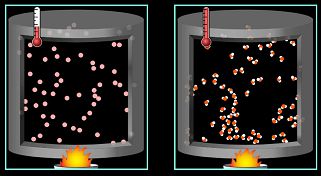
Thus, the combustion itself does not produce any sound, but due to the release of a high amount of energy, nearby molecules acquire a greater random kinetic energy which allows us to perceive a so-called Brownian noise.

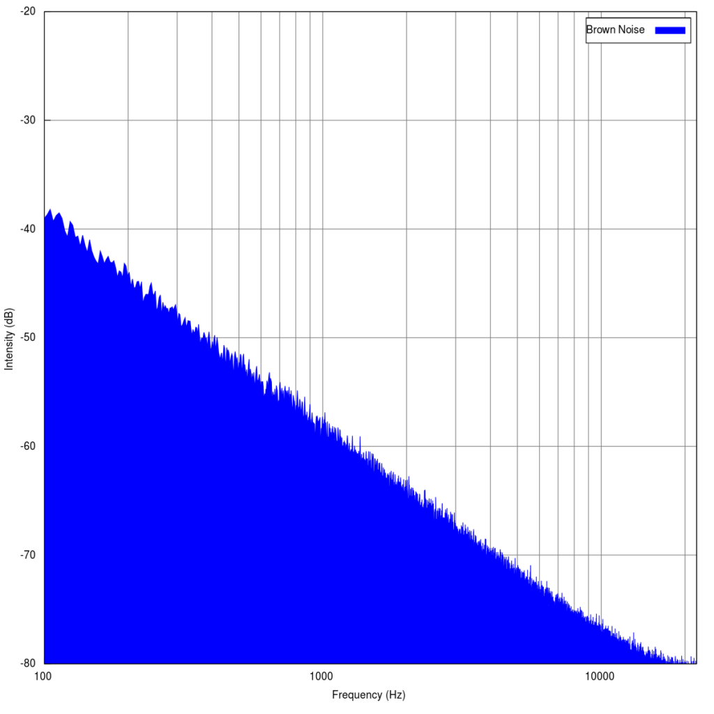
Brownian noise (or Brown Noise), is a noise characterized by the decrease of 6 dB per octave with increasing density.

Normally, we detect longitudinal waves, as they are made up of groups of particles that periodically oscillate with high amplitudes, so we can easily detect, for example, a human voice.

In the event of combustion due to the disorganized movement of the particles, the power at the eardrum is lower and this noise is not audible. This means that we mainly hear the popping of wood or the sound of the wind blowing as the air expands and rises.

Increasing the temperature leads to an increase in the average kinetic energy of the molecules, and thus increases the pressure.

Therefore, we could try to find the hypothetical temperature necessary for the Brownian noise produced by a fire to be audible.

In the work from Sivian and White [2] the minimum audible field (MAF) was determined, that is the thresholds for a tone presented in a sound field to a participant who is not wearing headphones.

Here we can also find a formula to express it:

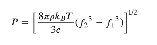
P is the RMS value, and we could consider it as P = 2 x 10^-2 (so 60 dB, as loud as a conversation);

𝜌 (Rho) is the density of air (1.225 kg/m^3);

kB is the Boltzmann constant (1.38064852 × 10^-23 m^2 kg s^-2 K^-1);

T is the temperature, in Kelvin

c is the speed of sound in air (344 m/s),

f1 and f2 are the frequency range. Let’s consider the audible range of 20-20000 Hz.

So we need to do the inverse formula to find T:

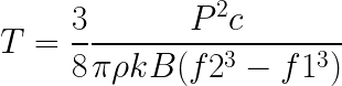
After all the calculations and after converting all the data to common values, the result is T= 88.144,20 K. An incredibly high temperature, much higher than the sun’s core! (5.778K)

Of course we can hear Brownian noise by simply generating it in any DAW and getting it to 60dB, yet we wouldn’t hear the noise caused by the random kinetic energy of air molecules.

References:

[2] L. J. Sivian, S.D. White. On minimum audible sound field. 2015.

Comparative Analysis of fake and proper Fact-Checking Sites #P1

This is an introduction to fact-checking sites and a clear definition of false information streams.

From politicians to marketers, from advocacy groups to brands — everyone who seeks to convince others has an incentive to distort, exaggerate or obfuscate the facts. This is why fact-checking has grown in relevance and has spread around the world in the recent decade.

According to a paper by Alexios Mantzarlis “MODULE 5 – Fact-checking 101” the type of fact-checking happens not before something is published but after a claim becomes of public relevance. This form of “ex post” fact-checking seeks to make politicians and other public figures accountable for the truthfulness of their statements. Fact-checkers in this line of work seek primary and reputable sources that can confirm or negate claims made to the public.

Alexios Mantzarlis also wrote about two moments, which were particularly significant to the growth of this journalistic practice. A first wave was kick-started by the 2009 Pulitzer Prize for national reporting, assigned to PolitiFact, a fact-checking project launched just over a year earlier by the St Petersburg Times (now Tampa Bay Times) in Florida. PolitiFact’s innovation was to rate claims on a “Truth-O-Meter”, adding a layer of structure and clarity to the fact checks.

Truth-O-Meter by PolitiFact

The second wave of fact-checking projects emerged following the global surge in so-called ‘fake news’. The term, now co-opted and misused, describes entirely fabricated sensationalist stories that reach enormous audiences by using social media algorithms to their advantage.

Vote Early False Information

This second wave often concentrated as much on fact-checking public claims as debunking these viral hoaxes. Debunking is a subset of fact-checking and requires a specific set of skills that are in common with verification.

The difference between Fact-checking and Verification

In part two an analysis and comparison of cloaked websites, which are sites published by individuals or groups who conceal authorship in order to
disguise deliberately a hidden political agenda, and fact-checking sites will be done. Therefore the websites will be compared on the basis of the following factors:

  1. User Experience (Survey about fact checking websites credibility)
  2. Design Differences (Typography, Images, etc.)
  3. Content (Expertise, Rigour, Transparency, Reliability)
  4. Overall Usability

Tabletop photography II

The tabletop photography gives photographers the chance to hone their craft and develop their abilities and skills regardless of time, weather and lighting situation. Lights, backgrounds, props-in short, everything that defines an picture are under the control of the creator, who can design scenes that range from objective to realistic to elaborate. 

Tabletop photography basics

Whether there is the intention to take pictures for products, foundation exposures for composite images, or you just want to capture a culinary scene, shoe-mount flashes can take you quite far.  These flash units are small, light, and battery operated. Therefore you don’t have to worry about extension cords and power outlets. But more important is the fact that these types of flashes are widespread. A lot of photographers have these flashes as a part of the basic equipment.

There are only a few things that influence the exposure of a photo. The focal length of the lens determines the perspective, the aperture defines the depth of field, the focus determines what will appear sharp in the picture and the lighting is basically the mood of an image. The advantage working in a studio means the photographer is in the position of being able to control all these factors and there are countless variations for exposing a single subject. 

Sharpness and Blur

Furthermore to determining the depth of field, the aperture also defines the degree of blur. Blur and sharpness have an quite big influence on the the look and vibe of the photography. As a result they could make an objective impression or otherwise a romantic impression. Because all elements of the tabletop shoot are under the control of the photographer, there is no limit to affect the sharpness and blur by changing the aperture. There is also the possibility to adjust the composition of the picture or the relative distances among each of the elements of the image. This means, for example, that an element can be placed by intention, beyond the depth of field to give the impression of a greater space or to separate the elements of the image more clearly. 

The distance of the main subject from the background of an image and the positioning of the focus lines during an exposure are of the utmost importance. They help you to develop the sense of space in your pictures, or in other words lead the viewer to pay attention to important details.

Focal length

The choice of focal length also affects the effect of an exposure. A wide angle lens makes objects in the foreground appear larger and allows you to include a larger background. In contrast, a telephoto lens compresses a photo to make it appear more compact and also shows less background in relation to the main subject of the image. A standard lens, often a macro lens for tabletop photography, displays objects the same way the human eye sees them, so it is useful for product shots where you want an objective perspective.

The wider the opening, the smaller the depth of field at which the subject appears acceptably sharp.

Light

The most important design tool of a photographer is light or the ability to change the quality of light through shapes. Shaping light in this sense has two meanings: First, photographers can shape the light themselves to be flat, pointed, hard, soft, scattered, etc. Second, light shapers enable photographers to stylize their subjects by modulating the lighting to match their photographic ideas. This is the exact process – what we call photography – that enables us to create two-dimensional images of objects based solely on the interplay of light and shadow.

Design with a purpose

Last but not least, a photographer’s creative instinct and effective composition are essential factors for a successful image. This includes choosing the right background, taking appropriate props and establishing a visual style that matches the subject/object. The photographer needs to stay objective when creating product shots and knowing when it is appropriate to use the photography to tell an emotional story.

When working professionally, the intended purpose of a photo should always be the primary influence on the visual design. The elaborate staging of a screw with multi-colored lighting and strong focus could work very well for the cover of a product catalog, but the same image would not be suitable for conveying objective information. To do this, it is better to make a clear product shot in which all the details of the screw are presented neutrally.

This also applies to the world of amateur photography, of course. Whether you are creating a product collection or taking a picture for an invitation, you should always consider the context in which the photo will be used and the effect the picture is going to have on the Person who sees it.

Know technology by heart

Proper use of the required technology requires both knowledge of how it works and a certain amount of experience from its regular use. The combination of this knowledge and experience helps to use the devices in a targeted and intuitive manner.

Therefore it is a great idea to set up some assignments for yourself from time to time and practice creating multiple photographic variations of the same subject. Your subject can be an everyday object staged under different lighting conditions, or it can be a broader theme, e.g. B. Representations of glass or transparent objects or even abstract images of aroma, coolness, softness or the like. Compare the results of the images you have created and determine which techniques have produced the best results.

After all, it is always good to ask yourself the following questions before starting a shoot:

– Will my plan achieve the desired result?

– Will the background and props serve the message you want?

– Are the subject and the background properly lit?

– Is the viewer’s gaze drawn to the important details of the picture?

– Does the selected focal length, perspective and depth of field match the subject?

– Is the focus on the optimal shot?

Quelle:

https://fixthephoto.com/tabletop-photography.html

https://www.amazon.de/dp/B00VB46CK6/ref=as_li_ss_tl?dchild=1&keywords=Tabletop+Photography+book&language=en_US&sr=8-1&linkCode=gs2&linkId=85d6c21259fd88d66db1bdb417f5376c&tag=expertphoto02-21&asin=B00VB46CK6&revisionId=4ce23c0c&format=1&depth=1

Realtime Automotive Rendering using Unreal Engine

Since PCs and especially their GPU-Units are getting more and more powerful, realtime rendering comes easier accessible for everyone. Rendering always has been very complex when it comes to absolute photorealism, but with realtime raytracing a milestone in terms of realsitic rendering has been set. The production of models, scene setup and shading is still very challenging, but with engines like Unity or Unreal, rendering is becoming less of a hassle as long rendering times are eliminated.

As an example of how powerful the Unreal Engine can be, I’ve attached two links from Duron Automotive, a professional 3D artist, with focus on realtime automotive renderings.

https://www.instagram.com/p/CLhcEI4i4Sy/
https://www.instagram.com/p/CLbgUOZiATf/

As the examples show, even the tiniest details like the structure of an aluminium surface inside of a car’s headlight, can be rendered perfectly. This opens up a totally new world with an encredibly hig level of detail.

https://www.instagram.com/p/CLEfJzupg6R/

This can be used to create videos, but also still images, which offer a grade of realism, where most people cannot tell the difference between a real photograph and a 3D rendered image.

Forms of therapy for people with prosopagnosia – Part 1

Short detour into how we humans actually perceive faces

There is a model that describes how we humans perceive faces. 
It happens in several phases and starts with the brain identifying something that looks like a human face. This is also the phase where we perceive basic visual things like size, figure-ground or orientation. After that, the face is mentally represented while at the same time the brain distinguishes what gender the person is and how old he or she is. In the next phase, the facial features that we perceive are compared with each face that we have stored in our brain and if the face matches we have the feeling that we recognize the person. After these phases we come to the fourth and last phase and we remember the name of the person.

Bruce and Young’s model of face-processing from 1986

Forms and treatments for Prosopagnosia 

People with this condition can see every detail of the face. The difference between the brains of these people and people who can recognize faces is that the collected impressions cannot be combined into a complete picture. Since no other cognitive areas in the brain are affected in prosopagnosia, it is not considered a disease. It is more of a dysfunction of the brain, or a genetically determined perceptual weakness. Therefore, the term face blindness is not actually correct, but is still often used to describe this condition.

Once again briefly as a repetition: aquired prosopagnosia develops by for example an accident or as a consequence of an illness, developmental prosopagnosia is since birth and remains in most cases a lifetime.
For simplicity, from here on aquired prosopagnosia will be shortened to AP and developmental prosopagnosia to DP.

As mentioned in my previous blog post, there is no guarantee of cure. The condition can improve, regardless of age or gender. However, if the damage to the brain is too great, no cure and little to no improvement is possible. Since every condition is different, all training programs must be customized to the person’s needs. Other important points to consider are: does the person only have problems recognizing faces or also objects. In the worst cases – apart from the typical consequences such as anxiety, difficulties with finding and practicing a job or generally social interaction with others – things such as food or doorknobs can no longer be recognized or it is necessary to learn to read and write again.

This image shows a brain scan of a 14 year old girl who was unable to recognize both faces and objects due to a medical condition when she was 8 years old. She had to relearn how to write and read.

There are many training programs that are supposed to help to remember faces or at least to be able to distinguish them. If therapies are actually successful, it is in most cases the fact that these effects do not last long and the therapy must be repeated after a few months. Interestingly, sometimes minor distinctions are made in the programs depending on what form of condition it is. This is because certain mechanisms in the brain, related to face processing, can be modified or changed, at least in people with DP.

Spoiler: Two specific cognitive training programs have been found to work best for AP and DP. One is face morph training and the other is holistic training. These two trainings were the most likely to show improvements.

(Next up in Part 2: Treatment approaches in acquired Prosopagnosia)

Sources

  1. Rehabilitation of face-processing skills in an adolescent with prosopagnosia: Evaluation of an online perceptual training programme, Sarah Bate, Rachel Bennetts, Joseph A. Mole, James A. Ainge, Nicola J. Gregory, Anna K. Bobak, Armanda Bussunt (04.11.2019), https://www.researchgate.net/publication/343935303_Prosopagnosia
  2. Approaches to Improving Face Processing in Prosopagnosia, Joe DeGutis (2016), https://www.cdnetwork.org/wp-content/uploads/2016/12/Degutis_12.13.pdf
  3. Face Processing Improvements in Prosopagnosia: Successes and Failures over the last 50 years, Joe DeGutis, Christopher Chiu, Mallory E Grosso, Sarah Cohan (8.2014), https://www.researchgate.net/publication/264940858_Face_Processing_Improvements_in_Prosopagnosia_Successes_and_Failures_over_the_last_50_years
  4. Face to Face Prosopagnosia Research & Community Spring 2020, o.A. (Spring 2020), https://www.faceblind.org/assets/files/newsletters/Face%20to%20Face%20Newsletter%20-%20Spring%202020.pdf

Das Ende des Loudness Wars?

Der renommierte Mastering-Ingenieur Bob Katz hat 2014 angekündigt, der Loudness War sei vorbei [1]. Und spätestens nach der Einführung von Streaming-Diensten, die eine automatisierte Lautheitsanpassung an Musikstücken vornehmen, um alle Musiktitel ungefähr gleich laut klingen zu lassen, könnte man behaupten, der Loudness War gehört der Vergangenheit an. Aber werden seit der Einführung von Lautheitsnormalisierungen auch tatsächlich wieder dynamischere Masterings erstellt und was genau ist der Loudness War?

Der sogenannte Loudness War beschreibt den seit den 80er Jahren andauernden Trend Musik in ihrer Dynamik immer stärker einzuschränken, um eine möglichst hohe Lautheit zu erzielen. Dabei basiert der Loudness War auf dem Phänomen, dass lautere Musikstücke im Vergleich zu leiseren als besser wahrgenommen werden, worauf Mastering-Ingenieure eine möglichst hohe Lautheit auf Kosten des Dynamikumfangs anstrebten, um sich so von der Konkurrenz abzuheben. [2]

Abbildung 1: Verlauf der durchschnittlichen Durchschnittspegel bzw. Dynamikumfänge von Musikstücken über die Jahre

Den Höhepunkt des Loudness Wars markiert das Album “Death Magnetic” von Metallica aus dem Jahr 2007, das einen großen medialen Aufschrei erzeugte, weil dessen Dynamikumfang so gering war, dass es von vielen Fans stark kritisiert wurde. Vor allem beim Vergleich mit der dynamischeren und weniger lauten Version desselben Songs im Videospiel Guitar Hero 3 zeigte sich, dass das offizielle Album-Mastering durch die extrem geringe Dynamik als schlechter wahrgenommen wird. Extrem komprimierte Musikstücke werden oft als “uninteressant”, “ermüdend” und “flach” beschrieben. [1, 3, 4]

Abbildung 2: Vergleich der Album Version des Songs “The Day That Never Comes” mit der Guitar Hero Version

Um dem Loudness War entgegenzuwirken hat die europäische Rundfunkunion Empfehlungen und Normen ausgesprochen, die dazu geführt haben, dass Programme und Werbungen bei vielen Radio- und Fernsehsendern wieder dynamischer wurden und geringere Lautheitswerte aufwiesen. [5]

Streaming-Dienste, wie Spotify, Apple Music, Youtube usw., haben eine automatische Lautheitsanpassung entwickelt, die die Lautheit eines Musikstücks misst und auf einen eigens definierten Wert regelt. Das hat zur Folge, dass Musikstücke, die einen deutlich höheren Lautheitswert aufweisen als der von den Streaming-Diensten festgelegte, um einen bestimmten Wert abgesenkt werden, sodass er mit dem definierten Wert übereinstimmt. Gemessen wird in einer speziell entwickelten Messskala für Lautheit, welche die Einheit LUFS (Loudness Units relative to Full Scale) festgelegt hat. [6, 7, 8]

Da Streaming inzwischen die populärste Form des Musikhörens ist, sollte dies eigentlich zur Folge haben, dass Mastering-Ingenieure in der heutigen Zeit Musikstücke wieder weniger stark komprimieren und einen höheren Dynamikumfang zulassen, da zu laute Musik ohnehin runterreguliert wird. [9]

Allerdings sieht man anhand der meisten populären Werke der letzten Jahre, dass viele Masterings dennoch stark komprimiert sind, um hohe Lautheiten zu erzielen. Vereinzelt gibt es allerdings auch in der Popmusik Ausnahmen, die den Schritt wagen, dynamischere Musiktitel zu veröffentlichen. Lady Gagas Song “Shallow”, der 2019 für einen Grammy nominiert wurde und auch ein weltweiter Erfolg wurde, zählt zu diesen. [10]

Quellen:

[1] https://www.soundonsound.com/techniques/end-loudness-war

[2] https://www.deutschlandfunknova.de/beitrag/loudness-war-lauter-ist-besser

[3] https://audiomunk.com/the-past-and-future-of-the-loudness-war/

[4] S. 18 https://unipub.uni-graz.at/obvugrhs/download/pdf/335378?originalFilename=true

[5] https://www.soundandrecording.de/tutorials/loudness-war-interview-mit-lautheitsforscher-rudi-ortner/

[6] https://www.bonedo.de/artikel/einzelansicht/spotify-und-das-ende-des-loudness-war.html

[7] https://blog.landr.com/de/was-sind-lufs-lautstaerkemessung-erklaert/

[8] https://artists.spotify.com/faq/mastering-and-loudness#my-track-doesn’t-sound-as-loud-as-other-tracks-on-spotify-why

[9] https://www.ifpi.org/our-industry/industry-data/

[10] https://www.nytimes.com/2019/02/07/opinion/what-these-grammy-songs-tell-us-about-the-loudness-wars.html


Bilderquellen:

Abbildung 1: S. 14 https://unipub.uni-graz.at/obvugrhs/download/pdf/335378?originalFilename=true

Abbildung 2: https://audiomunk.com/the-past-and-future-of-the-loudness-war/

Experimentelle Erkenntnisse des Effektes von Musik in der Werbung auf Aufmerksamkeit, Gedächtnis und Kaufintention (Allan, D. 2007)

Werbung und Musik wurden durch viele Studien bereits mit einer breiten Palette von Ergebnissen analysiert. Diese dabei erstellten Theorien und Modelle bilden die Grundlage der Musik in der Werbung und beinhalten unter anderem die Einstellungstheorie, die klassische Konditionierungstheorie, die Involvement-Theorie, das Elaboration-Likelihood-Modell (ELM), und die Musiktheorie.

Die Einstellungstheorie von Fishbein (1963) besagt, dass die Einstellung einer Person zu einem bestimmten Zeitpunkt, in einer bestimmten Situation, aus dem Gedächtnis aktiviert werden kann. Viele Forscher haben die Wirkung von Musik auf Einstellung gegenüber der Marke im Hinblick auf die Produktpräferenz (Allen & Madden, 1985; Gorn, 1982; Kellaris & Cox, 1989; Middlestadt et al., 1994; Park & Young, 1986; Pitt & Abratt, 1988; Zhu, 2005) und Kaufabsicht (Brooker & Wheatley, 1994; Morris & Boone, 1998) untersucht.

Die am meisten untersuchten Musikvariablen in Bezug auf die Einstellung zur Marke und zur Werbung sind die Indexikalität, d.h. “das Ausmaß, in dem die Musik emotionsgeladene Erinnerungen weckt”, und die Passung, d.h. “die Relevanz oder Angemessenheit der Musik zum Produkt oder zur zentralen Werbebotschaft” und ihre Wirkung auf die Verarbeitung der Werbung (MacInnis & Park, 1991).

Die Ergebnisse zweier Experimente unterstützen laut Gorn (1982) die Vorstellung, dass die einfache Assoziation zwischen einem Produkt und einem anderen Stimulus, wie Musik, die Produktpräferenzen, gemessen an der Produktwahl, beeinflussen kann. Außerdem wird ein Individuum, das sich in einem Entscheidungsmodus befindet, wenn es einem Werbespot ausgesetzt ist, stärker von den Informationen beeinflusst als ein Individuum, das sich nicht in einem Entscheidungsmodus befindet.

Viele Forscher haben versucht, Gorns Studie zu erweitern, waren aber nicht in der Lage, seine Ergebnisse zu replizieren (Allen & Madden, 1985; Alpert & Alpert, 1990, Kellaris & Cox, 1989; Pitt & Abratt, 1988).

Krugman (1965) definierte Involvement (Involvement Modell) als “die Anzahl der bewussten Brückenerfahrungen, Verbindungen oder persönlichen Bezüge pro Minute, die ein Zuschauer zwischen seinem eigenen Leben und einem Stimulus herstellt” (S. 356). Salmon (1986) fügte hinzu, dass “Involvement, in welcher Form auch immer, sowohl den Erwerb als auch die Verarbeitung von Informationen zu vermitteln scheint, indem es einen erhöhten Erregungszustand und/oder eine größere kognitive Aktivität in einer Interaktion zwischen einer Person und einem Stimulus aktiviert” (S. 264). ELM geht davon aus, dass sobald ein Individuum eine Nachricht erhält, die Verarbeitung beginnt. Abhängig von der persönlichen Relevanz dieser Information, wird der Empfänger einer von zwei “Routen” zur Überzeugung folgen: “zentral” und “peripher”. Wenn der Konsument der Botschaft einen hohen Grad an Aufmerksamkeit schenkt, besteht ein hohes Involvement und damit eine zentrale (aktive) Verarbeitungsroute.

Wenn der Konsument der Botschaft einen geringen Grad an Aufmerksamkeit schenkt, liegt ein geringes Involvement und ein peripheren (passiven) Verarbeitungsweg. Petty und Cacioppo (1986) vermuteten, dass hohes Involvement das Ergebnis einer Botschaft mit hoher persönlicher Relevanz ist.

Macklin (1988) fand außerdem heraus, dass Botschaften, die in einem produzierten, originellen Jingle gesungen wurden, der sich wie ein Kinderlied anhörte, bei Kindern die gleiche Erinnerung hervorriefen wie gesprochene Botschaften.

Variablen (nach Allan, 2007):

  1. Haltung gegenüber der Anzeige                             Music fit

2. Dauer der Anzeige                                                     Erregung durch die Musik

3. Haltung zur Marke                                                    Attraktivität der
Musik/Präsenz

4. Erinnerung an die Marke                                        Music fit, Melodie, Tempo,
Präsenz

5. Vergnügen/ Erregung                                                Tempo, Textur, Tonalität

6. Kauf                                                                           Gefühl, Platzierung,
Tempo, Präsenz

7.Intention                                                                    Melodie, Music fit,
Platzierung, Modalität

Quellen:

Allan, D. (2007). Sound Advertising: A Review of the Experimental Evidence on the Effects of Music in Commercial on Attention, Memory, Attitudes and Purchase Intention. Journal of Media Psychology. Volume 12, Nr. 3

Allen, C. T., & Madden, T. J. (1985). A closer look at classical conditioning. Journal of Consumer Research, 12(3), 301-315.

Alpert, J. L, & Alpert, M. I. (1990). Music influences on mood and purchase intentions. Psychology & Marketing, 7(2), 109-133.

Fishbein, M. (1963). An investigation of the relationship between beliefs about an object and the attitude toward the object. Human Relations, 16, 233-240.

Gorn, G. J. (1982). The effects of music in advertising on choice behavior: A classical conditioning approach. Journal of Marketing, 46, 94-101.

Kellaris, J. J., & Cox, A. D. (1989). The effects of background music in advertising: A reassessment. Journal of Consumer Research, 16, 113-118.

Krugman, H. E. (1965). The impact of television advertising: Learning without involvement. Public Opinion Quarterly, 29, 349-356.

MacInnis, D. J., & Park, C. W. (1991). The differential role of characteristics of music on high- and low-involvement consumers’ processing of ads. Journal of Consumer Research, 18, 161-173.

Macklin, M. C. (1988). The relationship between music in advertising and children’s responses: an experimental investigation. In S. Hecker & D. W. Stewart (Eds.), Nonverbal Communication in Advertising (pp. 225-245). Lexington, MA: Lexington Books.

Middlestadt, S. E., Fishbein, M., & Chan, D. K.-S. (1994). The effect of music on brand attitudes: Affect- or belief-based change? In E. M. Clark & T. C. Brock & D. W. Stewart (Eds.), Attention, Attitude, and Affect in Response to Advertising (pp. 149-167). Hillsdale, NJ:

Park, C. W., & Young, S. M. (1986). Consumer response to television commercials: The impact of involvement and background music on brand attitude formation. Journal of Marketing Research, 23, 11-24.

Petty, R. E., & Cacioppo, J. T. (1986). Communication and persuasion: Central and peripheral routes to attitudes change. New York: Springer-Verlag.

Pitt, L. F., & Abratt, R. (1988). Music in advertisements for unmentionable products – a classical conditioning experiment. International Journal of Advertising, 7(2), 130-137.   

Salmon, C. (1986). Perspectives on involvement in consumer and communication research. In B. Dervin (Ed.), Progress in Communication Sciences (Vol. 7, pp. 243-268). Norwood, NJ: Ablex.

Wheatley, J. J., & Brooker, G. (1994). Music and spokesperson effects on recall and cognitive response to a radio advertisement. In E. M. Clark & T. C. Brock & D. W. Stewart (Eds.), Attention, Attitude, and Affect in Response to Advertising (pp. 189-204). Hillside, NJ: Lawrence Erlbaum Associates, Inc.

Zhu, R., & Meyers-Levy. (2005). Distinguishing between meanings of music: When background music affects product perceptions. Journal of Marketing Research, 42, 333-345.

Analog/Digital – RGB Print

As recently mentioned in the entry about colours for digital and analog media there are two different color systems in use. While for digital applications the system is of additive nature (=the sum of colours will show a white display), the analog use of colours is of subtractive nature (=adding and mixing colours will end up in black colour).

Thus in print production it seemed impossible to represent the RGB color space that obviously contains a broader variety of colours than the CMYK, Pantone or any other subtractive colour system used for printing.

This fact has changed recently: referring to the article on Page magazine about Swiss screen printer Lorenz Boegli, there are special colours for screen print which are capable of representing the RGB colour space.

When Boegli used the Spectraval™ pearlescent pigments by Merck, he found out that the colours turn into a tertiary colour when overprinting them. Red on blue turned magenta, green on red turned yellow. His logic conclusion was that the sum of red, green and blue has to turn out white – and that’s just what happened.

However the revolutionary RGB-printing for now works only with screen printing and also only on black backgrounds. The reason for this is that the reflective power of the pigments only gets visible on black – on white paper the colours are more or less invisible.

Of course the RGB printing result is not exactly what would be emitted by screens – the pictures seem quite metallic and silverish. Additionally not only a lot of printing experience but also a suitable picture and the surface you print on has an effect on the result. But still it gets close and the system is the same, opening the addtive colour system to the analog world.

Full article: https://page-online.de/tools-technik/rgb-drucken/
More about Spectraval™ Colours: Merck Group

Bela Board

The Bela Board lets you create different interactions with sensors and sounds. It is built to interact with various inputs for example touch sensors or an accelerometer. The Bela Mini which I am using in my project features 16 digital I/O channels, 8 analog inputs and 2 audio input and output channels. The Bela board is accessed via the Bela software that you can use via the browser and communicate with the board while connected via USB. With this method it is very easy to load the Pure Data patches onto the Bela board. To point out one disadvantage is, that you can’t edit the patch directly on the board, you have to upload it every time if you change something. (Bela, 2021)

Bela mini: Audioboard jetzt im Mini-Format | heise online
Source: bela.io

Processing Audio Data for Use in Machine Learning with Python

I am currently working on a project where I am using machine learning to generate audio samples. One of the steps involved is pre-processing.

What is pre-processing?

Pre-processing is a process where input data somehow gets modified to be more handleable. An easy everyday life example would be packing items in boxes to allow for easier storing. In my case, I use pre-processing to make sure all audio samples are equal before further working with them. By equal, in this case I mean same sample rate, same file type, same length and same time of peak. This is important because having a huge mess of samples makes it much harder for the algorithm to learn the dataset and not just return random noise but actually similar samples.

The Code: Step by step

First, we need some samples to work with. Once downloaded and stored somewhere we need to specify a path. I import os to store the path like so:


import os


PATH = r"C:/Samples"

DIR = os.listdir( PATH )


 Since we are already declaring constants, we can add the following:

ATTACK_SEC = 0.1

LENGTH_SEC = 0.4

SAMPLERATE = 44100


 These are the “settings” for our pre-processing script. The values depend strongly on our data so when programming this on your own, try to figure out yourself what makes sense and what does not.

Instead of ATTACK_SEC we could use ATTACK_SAMPLES as well, but I prefer to calculate the length in samples from the data above:

import numpy as np


attack_samples = int(np.round(ATTACK_SEC * SAMPLERATE, 0))

length_samples = int(np.round(LENGTH_SEC * SAMPLERATE, 0))


 One last thing: Since we usually do not want to do the pre-processing only once, form now on everything will run in a for-loop:

for file in DIR:


 Because we used the os import to store the path, every file in the directory can now simply accessed by the file variable.

Now the actual pre-processing begins. First, we make sure that we get a 2D array whether it is a stereo file or a mono file. Then we can resample the audio file with librosa.

import librosa

import soundfile as sf


try:

data, samplerate = sf.read(PATH + "/" + file, always_2d = True)

except:

continue


data = data[:, 0]

sample = librosa.resample(data, orig_sr=samplerate, target_sr=SAMPLERATE)


 The next step is to detect a peak and to align it to a fixed time. The time-to-peak is set by our constant ATTACK_SEC and the actual peak time can be found with numpy’s argmax. Now we only need to compare the two values and do different things depending on which is bigger:

peak_timestamp = np.argmax(np.abs(sample))


if (peak_timestamp > attack_samples):

new_start = peak_timestamp  attack_samples

processed_sample = sample[new_start:]


elif (peak_timestamp < attack_samples):

gap_to_start = attack_samples  peak_timestamp

processed_sample = np.pad(sample, pad_width=[gap_to_start, 0])


else:

processed_sample = sample


 And now we do something very similar but this time with the LENGTH_SEC constant:

if (processed_sample.shape[0] > length_samples):

processed_sample = processed_sample[:length_samples]


elif (processed_sample.shape[0] < length_samples):

cut_length = length_samples  processed_sample.shape[0]

processed_sample = np.pad(processed_sample, pad_width=[0, cut_length])


else:

processed_sample = processed_sample


 Note that we use the : operator to cut away parts of the samples and np.pad() to add silence to either the beginning or the end (which is defined by the location of the 0 in pad_width=[]).

With this the pre-processing is done. This script can be hooked into another program right away, which means you are done. But there is something more we can do. The following addition lets us preview the samples and the processed samples both via a plot and by just playing them:

import sounddevice as sd

import time

import matplotlib.pyplot as plt


#PLOT & PLAY


plt.plot(sample)

plt.show()

time.sleep(0.2)

sd.play(sample)

sd.wait()


plt.plot(processed_sample)

plt.show()

time.sleep(0.2)

sd.play(processed_sample)

sd.wait()


 Alternatively, we can also just save the files somewhere using soundfile:

sf.write(os.path.join(os.path.join(PATH, "preprocessed"), file), processed_sample, SAMPLERATE, subtype='FLOAT')


 And now we are really done. If you have any comments or suggestions leave them down below!