Sensors Part I: Accelerometer

An accelerometer measures the acceleration of an object, or in other words the rate of change of an objects velocity. It also uses earth`s gravity on a static object and measures its movement or vibrations. The most typical sensors have 3 axes, oriented on the x, y and z planes. One of the most common usages of accelerometer would be the orientation sensor in smart phones.

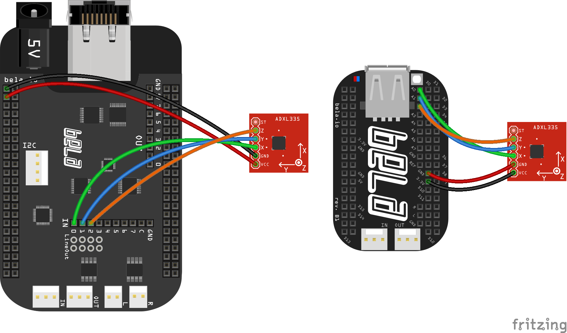
As we already know, accelerometers are analog sensors that provide a different amount of voltage for each axes. To connect it to the bela we need 5 wires, 3 for the axes, one for the power and the last one for the Ground.

Connecting Accelerometer to Bela Board; Source: bela.io

Radiohead & Ondes Martenot

At the beginning of the XX century many electronic instruments have been invented, some have had better luck than others, and one of these unlucky ones is the Ondes Martenot.

This instrument was invented in 1928 by Maurice Martenot, a French cellist.

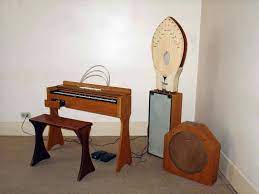
But what is it? It is somewhat of a cross between an Organ and a Theremin.

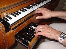
Originally, the main interface was a metal ring, which the player worn in the right index finger. The movement of the finger (up and down a wire) creates a theremin-like tone. Then a four-octave keyboard was added, yet not a normal one, because it has moveable keys that create a vibrato when wiggled. All this is enclosed in a wooden frame that features a drawer that allows manipulation of volume and timbre by the left hand. Volume is controlled with a touch-sensitive glass “lozenge”, called the “gradation key”; the further the lozenge is depressed, the louder the volume.

Early models produce only a few waveforms. Later models can simultaneously generate sine, peak-limited triangle, square, pulse, and full-wave rectified sine waves, in addition to pink noise, all controlled by switches in the drawer.

The inventor was fascinated by the accidental overlapping of tones of military radio oscillators and wanted to build an instrument to replicate it, but with the same tonal expression as a cello.

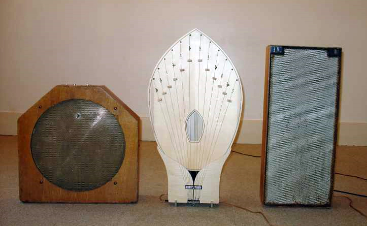
Four speakers were produced for the instrument, called “diffuseurs”.

The “Métallique” (imm. below, first from left) features a gong instead of a speaker cone, producing a metallic timbre.

The “Palme” speaker (imm. below, middle), has a resonance chamber laced with strings tuned to all 12 semitones of an octave; when a note is played in tune, it resonates a particular string, producing chiming tones

The last one is a normal cabinet.

It has been used by composers such as Edgar Varèse, Pierre Boulez and Olivier Messiaen, but its “rebirth” in the modern era and its diffusion in the context of popular music can be attributed to Jonny Greenwood, best known for his role as a guitarist in Radiohead .

Jonny, visionary musician and creator of a new way of thinking and playing music, was so fascinated by the Ondes Martenot that he decided to integrate them into Radiohead’s music. This “journey” began with their amazing album Kid A (2000) and has been played on some of their most important songs ever since. In live performances of their song Weird Fishes/Arpeggi they even use a group of six ondes martenot.

Here is a collection of Radiohead’s songs with Ondes Martenot

Greenwood also wrote Smear, a piece for two Ondes Martenot:

Thanks to Jonny Greenwood it has had a new light and has found many applications in modern popular music. For example, Yann Tiersen used it for the Amelie soundtrack and Thomas Bloch, Ondes Martenot virtuoso, also played it on records by Tom Waits, Marianne Faithfull and in Damon Albarn’s Monkey: Journey to the West Opera.

References

[1] Wikipedia – Ondes Martenot.

[2] The Guardian – Hey, what’s that sound: Ondes martenot.

[3] Britannica – Ondes martenot.

Fulldome

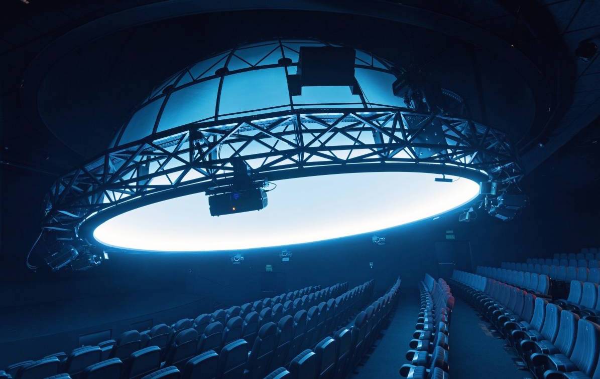
Brno Planetarium, Czech Republic
Brno Observatory & Planetarium

What does “Fulldome” mean?

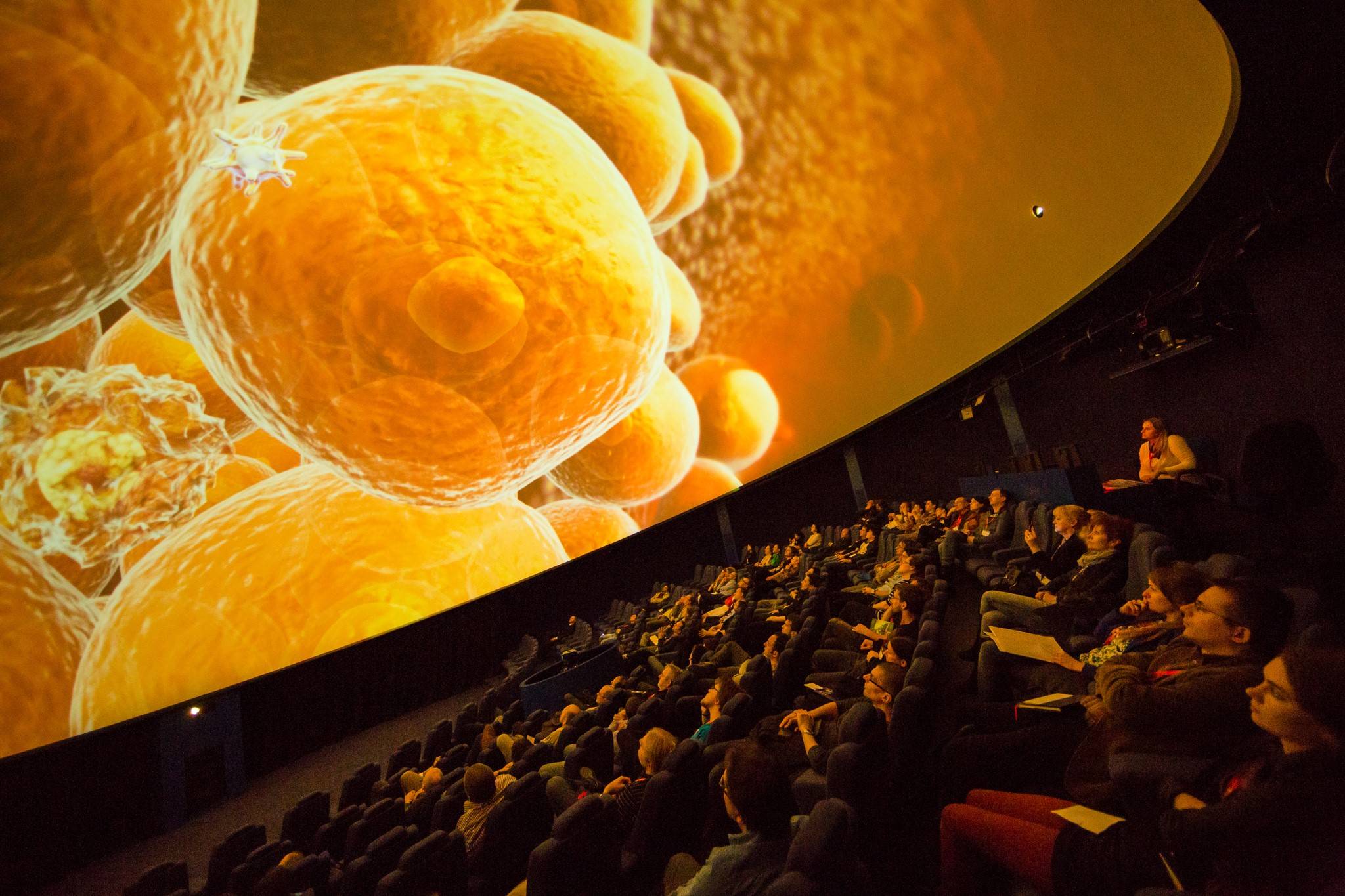
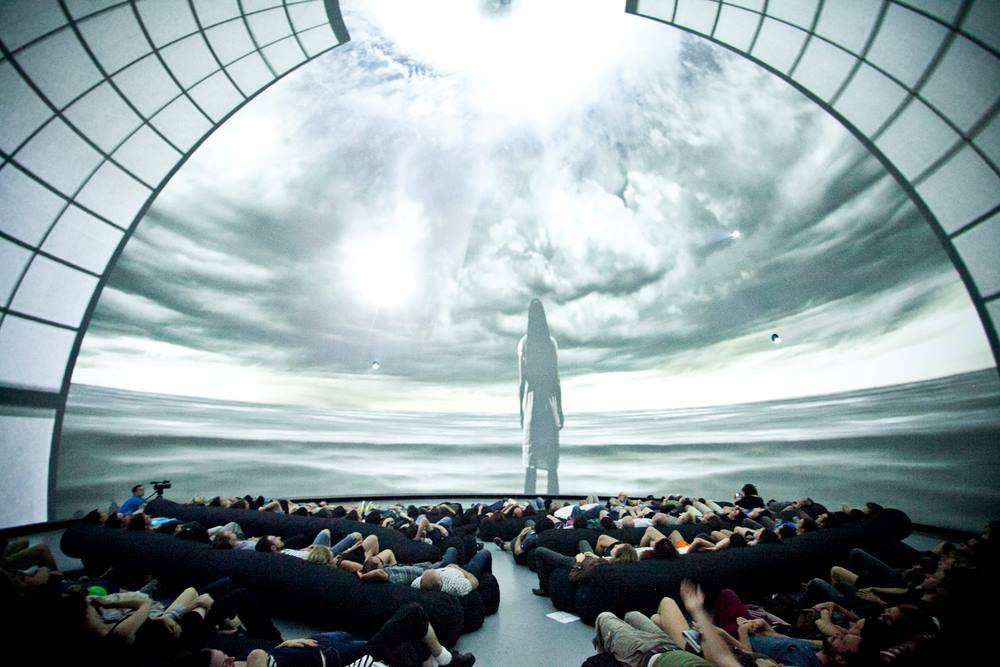
Fulldome refers to immersive dome-based video projection environments where the viewer is surrounded by the video projection in a hemispherical angle of view.

The dome, horizontal or tilted, is filled with real-time (interactive) or pre-rendered (linear) computer animations, live capture images, or composited environments. Even though astronomy is the most common topic, there are no content limitations and it’s now used also for entertaining shows and other hyper-realistic presentations.Brno Planetarium, Czech Republic Morrison Planetarium
California Academy of Sciences

Developement

Although the current technology emerged in the early-to-mid 1990’s (USA and Japan), fulldome environments have evolved from numerous influences, including immersive art and storytelling, with technological roots in domed architecture, planetariums, multi-projector film environments, flight simulation, and virtual reality.

Early live-action dome cinemas used wide-angle lenses and 35- or 70-mm filmstock. There are still around 125 giant screen dome cinemas operating in the world. However the expense and ungainly nature of the giant screen film medium has prevented more widespread use. Also, film formats such as Omnimax (Imax Dome) do not cover the entire dome surface, leaving the rear section of the dome blank (though, due to seating arrangements, that part of the dome was not seen by most viewers).

Early approaches to fulldome video projection utilized monochromatic vector graphics systems projected through a fisheye lens. Contemporary configurations employ raster video projectors, either single projectors with wide-angle lenses or multiple edge-blended projectors to cover the dome surface with high-resolution, full-color imagery.Planetarium Venus, Poland Planetarium Wenus
Kepler Science Center

A great fast-growing immersive

The fulldome experience comes out as one of the most immersive and entertaining ways to engage a wide range of people with a limitless scope of applications, including education, arts, games and wellness.

Fulldome media is experiencing enormous growth with new planetariums and digital theatres being built around the world, reaching out to new audiences to make them fall in love with such beautiful technology.Société des Arts Technologiques, Canada IX Symposium
Société des Arts Technologiques

Analog/Digital Input – Bela Board into Pure Data

Analog Input

Analog signals can vary anywhere between 0 and 1, whereas digital signals on the Bela have only two states (0, 1). In my project I am using two different types of analog sensors, which are an accelerometer and two potentiometers. I will explain them in more detail afterwards. With these analog inputs you can have a variable control over some parameters and tune them exactly like you want them to be. (Bela, 2021)

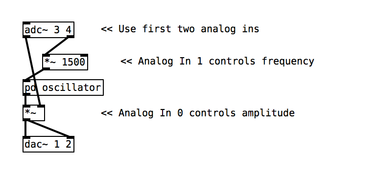
To read from the analog inputs in Pure Data an adc~ object is needed. The incoming signals are sampled at audio sampling rate, so that you can handle them in the same way as audio signals.

Analog Input in PD; Source: bela.io

Digital Input

As mentioned above, the digital inputs have only two states and are perfect suitable for push buttons. The digital port has to be configured as an input or output. To use a push button it has to be an input of course. If the button is pressed, the input receives the incoming 3.3 volts, and 0 V when its off. In the following example in Pure Data, digital pin 18 is set as an input and pin 17 as an output. (Bela, 2021)

Digital Input in PD; Source: bela.io

Sound of Fire?

What is really the sound of fire? In general, the fire should not make any sound, what we hear is more the burning object or the air itself, the so-called crackling and hissing.

Sound is defined as oscillation in pressure, particle displacement and velocity propagated in medium such as air or water, that have density.

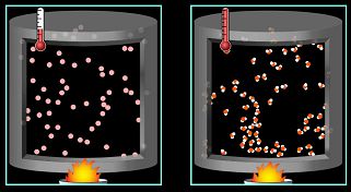
On the other hand, thermal conduction, hence the transfer of heat (energy) resulting from temperature differences, occurs through the random movement of atoms or molecules.

Heat is vibration of molecules, but it takes a very large amount of molecules moving organized together to create what we perceive as sound, as we perceive the vibration of the air as a whole, not of individual molecules.

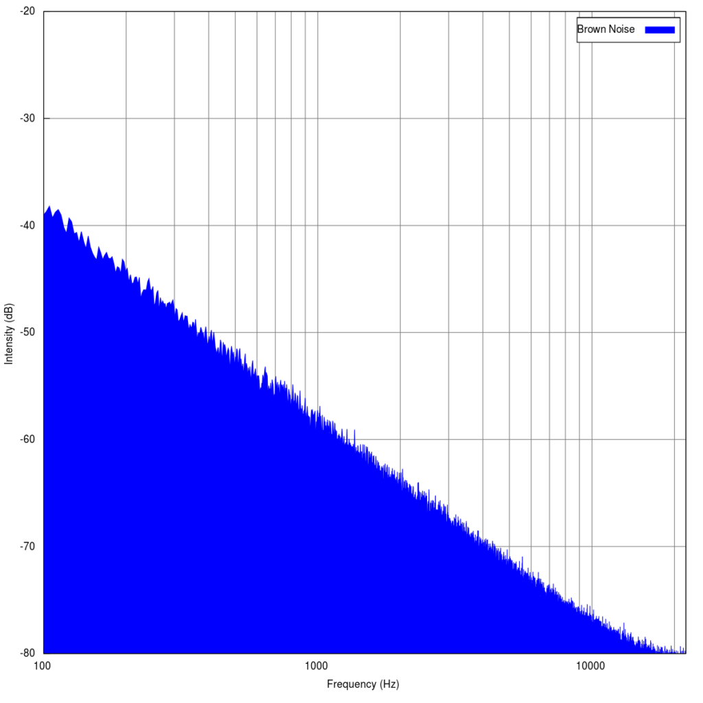
Thus, the combustion itself does not produce any sound, but due to the release of a high amount of energy, nearby molecules acquire a greater random kinetic energy which allows us to perceive a so-called Brownian noise.

Brownian noise (or Brown Noise), is a noise characterized by the decrease of 6 dB per octave with increasing density.

Normally, we detect longitudinal waves, as they are made up of groups of particles that periodically oscillate with high amplitudes, so we can easily detect, for example, a human voice.

In the event of combustion due to the disorganized movement of the particles, the power at the eardrum is lower and this noise is not audible. This means that we mainly hear the popping of wood or the sound of the wind blowing as the air expands and rises.

Increasing the temperature leads to an increase in the average kinetic energy of the molecules, and thus increases the pressure.

Therefore, we could try to find the hypothetical temperature necessary for the Brownian noise produced by a fire to be audible.

In the work from Sivian and White [2] the minimum audible field (MAF) was determined, that is the thresholds for a tone presented in a sound field to a participant who is not wearing headphones.

Here we can also find a formula to express it:

P is the RMS value, and we could consider it as P = 2 x 10^-2 (so 60 dB, as loud as a conversation);

𝜌 (Rho) is the density of air (1.225 kg/m^3);

kB is the Boltzmann constant (1.38064852 × 10^-23 m^2 kg s^-2 K^-1);

T is the temperature, in Kelvin

c is the speed of sound in air (344 m/s),

f1 and f2 are the frequency range. Let’s consider the audible range of 20-20000 Hz.

So we need to do the inverse formula to find T:

After all the calculations and after converting all the data to common values, the result is T= 88.144,20 K. An incredibly high temperature, much higher than the sun’s core! (5.778K)

Of course we can hear Brownian noise by simply generating it in any DAW and getting it to 60dB, yet we wouldn’t hear the noise caused by the random kinetic energy of air molecules.

References:

[2] L. J. Sivian, S.D. White. On minimum audible sound field. 2015.

Das Ende des Loudness Wars?

Der renommierte Mastering-Ingenieur Bob Katz hat 2014 angekündigt, der Loudness War sei vorbei [1]. Und spätestens nach der Einführung von Streaming-Diensten, die eine automatisierte Lautheitsanpassung an Musikstücken vornehmen, um alle Musiktitel ungefähr gleich laut klingen zu lassen, könnte man behaupten, der Loudness War gehört der Vergangenheit an. Aber werden seit der Einführung von Lautheitsnormalisierungen auch tatsächlich wieder dynamischere Masterings erstellt und was genau ist der Loudness War?

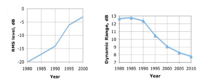
Der sogenannte Loudness War beschreibt den seit den 80er Jahren andauernden Trend Musik in ihrer Dynamik immer stärker einzuschränken, um eine möglichst hohe Lautheit zu erzielen. Dabei basiert der Loudness War auf dem Phänomen, dass lautere Musikstücke im Vergleich zu leiseren als besser wahrgenommen werden, worauf Mastering-Ingenieure eine möglichst hohe Lautheit auf Kosten des Dynamikumfangs anstrebten, um sich so von der Konkurrenz abzuheben. [2]

Abbildung 1: Verlauf der durchschnittlichen Durchschnittspegel bzw. Dynamikumfänge von Musikstücken über die Jahre

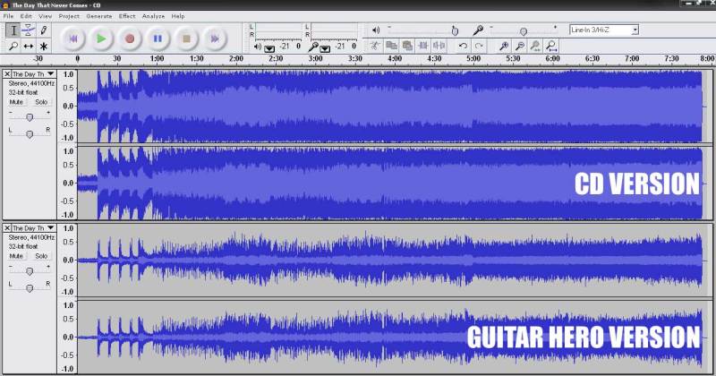
Den Höhepunkt des Loudness Wars markiert das Album “Death Magnetic” von Metallica aus dem Jahr 2007, das einen großen medialen Aufschrei erzeugte, weil dessen Dynamikumfang so gering war, dass es von vielen Fans stark kritisiert wurde. Vor allem beim Vergleich mit der dynamischeren und weniger lauten Version desselben Songs im Videospiel Guitar Hero 3 zeigte sich, dass das offizielle Album-Mastering durch die extrem geringe Dynamik als schlechter wahrgenommen wird. Extrem komprimierte Musikstücke werden oft als “uninteressant”, “ermüdend” und “flach” beschrieben. [1, 3, 4]

Abbildung 2: Vergleich der Album Version des Songs “The Day That Never Comes” mit der Guitar Hero Version

Um dem Loudness War entgegenzuwirken hat die europäische Rundfunkunion Empfehlungen und Normen ausgesprochen, die dazu geführt haben, dass Programme und Werbungen bei vielen Radio- und Fernsehsendern wieder dynamischer wurden und geringere Lautheitswerte aufwiesen. [5]

Streaming-Dienste, wie Spotify, Apple Music, Youtube usw., haben eine automatische Lautheitsanpassung entwickelt, die die Lautheit eines Musikstücks misst und auf einen eigens definierten Wert regelt. Das hat zur Folge, dass Musikstücke, die einen deutlich höheren Lautheitswert aufweisen als der von den Streaming-Diensten festgelegte, um einen bestimmten Wert abgesenkt werden, sodass er mit dem definierten Wert übereinstimmt. Gemessen wird in einer speziell entwickelten Messskala für Lautheit, welche die Einheit LUFS (Loudness Units relative to Full Scale) festgelegt hat. [6, 7, 8]

Da Streaming inzwischen die populärste Form des Musikhörens ist, sollte dies eigentlich zur Folge haben, dass Mastering-Ingenieure in der heutigen Zeit Musikstücke wieder weniger stark komprimieren und einen höheren Dynamikumfang zulassen, da zu laute Musik ohnehin runterreguliert wird. [9]

Allerdings sieht man anhand der meisten populären Werke der letzten Jahre, dass viele Masterings dennoch stark komprimiert sind, um hohe Lautheiten zu erzielen. Vereinzelt gibt es allerdings auch in der Popmusik Ausnahmen, die den Schritt wagen, dynamischere Musiktitel zu veröffentlichen. Lady Gagas Song “Shallow”, der 2019 für einen Grammy nominiert wurde und auch ein weltweiter Erfolg wurde, zählt zu diesen. [10]

Quellen:

[1] https://www.soundonsound.com/techniques/end-loudness-war

[2] https://www.deutschlandfunknova.de/beitrag/loudness-war-lauter-ist-besser

[3] https://audiomunk.com/the-past-and-future-of-the-loudness-war/

[4] S. 18 https://unipub.uni-graz.at/obvugrhs/download/pdf/335378?originalFilename=true

[5] https://www.soundandrecording.de/tutorials/loudness-war-interview-mit-lautheitsforscher-rudi-ortner/

[6] https://www.bonedo.de/artikel/einzelansicht/spotify-und-das-ende-des-loudness-war.html

[7] https://blog.landr.com/de/was-sind-lufs-lautstaerkemessung-erklaert/

[8] https://artists.spotify.com/faq/mastering-and-loudness#my-track-doesn’t-sound-as-loud-as-other-tracks-on-spotify-why

[9] https://www.ifpi.org/our-industry/industry-data/

[10] https://www.nytimes.com/2019/02/07/opinion/what-these-grammy-songs-tell-us-about-the-loudness-wars.html


Bilderquellen:

Abbildung 1: S. 14 https://unipub.uni-graz.at/obvugrhs/download/pdf/335378?originalFilename=true

Abbildung 2: https://audiomunk.com/the-past-and-future-of-the-loudness-war/

Experimentelle Erkenntnisse des Effektes von Musik in der Werbung auf Aufmerksamkeit, Gedächtnis und Kaufintention (Allan, D. 2007)

Werbung und Musik wurden durch viele Studien bereits mit einer breiten Palette von Ergebnissen analysiert. Diese dabei erstellten Theorien und Modelle bilden die Grundlage der Musik in der Werbung und beinhalten unter anderem die Einstellungstheorie, die klassische Konditionierungstheorie, die Involvement-Theorie, das Elaboration-Likelihood-Modell (ELM), und die Musiktheorie.

Die Einstellungstheorie von Fishbein (1963) besagt, dass die Einstellung einer Person zu einem bestimmten Zeitpunkt, in einer bestimmten Situation, aus dem Gedächtnis aktiviert werden kann. Viele Forscher haben die Wirkung von Musik auf Einstellung gegenüber der Marke im Hinblick auf die Produktpräferenz (Allen & Madden, 1985; Gorn, 1982; Kellaris & Cox, 1989; Middlestadt et al., 1994; Park & Young, 1986; Pitt & Abratt, 1988; Zhu, 2005) und Kaufabsicht (Brooker & Wheatley, 1994; Morris & Boone, 1998) untersucht.

Die am meisten untersuchten Musikvariablen in Bezug auf die Einstellung zur Marke und zur Werbung sind die Indexikalität, d.h. “das Ausmaß, in dem die Musik emotionsgeladene Erinnerungen weckt”, und die Passung, d.h. “die Relevanz oder Angemessenheit der Musik zum Produkt oder zur zentralen Werbebotschaft” und ihre Wirkung auf die Verarbeitung der Werbung (MacInnis & Park, 1991).

Die Ergebnisse zweier Experimente unterstützen laut Gorn (1982) die Vorstellung, dass die einfache Assoziation zwischen einem Produkt und einem anderen Stimulus, wie Musik, die Produktpräferenzen, gemessen an der Produktwahl, beeinflussen kann. Außerdem wird ein Individuum, das sich in einem Entscheidungsmodus befindet, wenn es einem Werbespot ausgesetzt ist, stärker von den Informationen beeinflusst als ein Individuum, das sich nicht in einem Entscheidungsmodus befindet.

Viele Forscher haben versucht, Gorns Studie zu erweitern, waren aber nicht in der Lage, seine Ergebnisse zu replizieren (Allen & Madden, 1985; Alpert & Alpert, 1990, Kellaris & Cox, 1989; Pitt & Abratt, 1988).

Krugman (1965) definierte Involvement (Involvement Modell) als “die Anzahl der bewussten Brückenerfahrungen, Verbindungen oder persönlichen Bezüge pro Minute, die ein Zuschauer zwischen seinem eigenen Leben und einem Stimulus herstellt” (S. 356). Salmon (1986) fügte hinzu, dass “Involvement, in welcher Form auch immer, sowohl den Erwerb als auch die Verarbeitung von Informationen zu vermitteln scheint, indem es einen erhöhten Erregungszustand und/oder eine größere kognitive Aktivität in einer Interaktion zwischen einer Person und einem Stimulus aktiviert” (S. 264). ELM geht davon aus, dass sobald ein Individuum eine Nachricht erhält, die Verarbeitung beginnt. Abhängig von der persönlichen Relevanz dieser Information, wird der Empfänger einer von zwei “Routen” zur Überzeugung folgen: “zentral” und “peripher”. Wenn der Konsument der Botschaft einen hohen Grad an Aufmerksamkeit schenkt, besteht ein hohes Involvement und damit eine zentrale (aktive) Verarbeitungsroute.

Wenn der Konsument der Botschaft einen geringen Grad an Aufmerksamkeit schenkt, liegt ein geringes Involvement und ein peripheren (passiven) Verarbeitungsweg. Petty und Cacioppo (1986) vermuteten, dass hohes Involvement das Ergebnis einer Botschaft mit hoher persönlicher Relevanz ist.

Macklin (1988) fand außerdem heraus, dass Botschaften, die in einem produzierten, originellen Jingle gesungen wurden, der sich wie ein Kinderlied anhörte, bei Kindern die gleiche Erinnerung hervorriefen wie gesprochene Botschaften.

Variablen (nach Allan, 2007):

  1. Haltung gegenüber der Anzeige                             Music fit

2. Dauer der Anzeige                                                     Erregung durch die Musik

3. Haltung zur Marke                                                    Attraktivität der
Musik/Präsenz

4. Erinnerung an die Marke                                        Music fit, Melodie, Tempo,
Präsenz

5. Vergnügen/ Erregung                                                Tempo, Textur, Tonalität

6. Kauf                                                                           Gefühl, Platzierung,
Tempo, Präsenz

7.Intention                                                                    Melodie, Music fit,
Platzierung, Modalität

Quellen:

Allan, D. (2007). Sound Advertising: A Review of the Experimental Evidence on the Effects of Music in Commercial on Attention, Memory, Attitudes and Purchase Intention. Journal of Media Psychology. Volume 12, Nr. 3

Allen, C. T., & Madden, T. J. (1985). A closer look at classical conditioning. Journal of Consumer Research, 12(3), 301-315.

Alpert, J. L, & Alpert, M. I. (1990). Music influences on mood and purchase intentions. Psychology & Marketing, 7(2), 109-133.

Fishbein, M. (1963). An investigation of the relationship between beliefs about an object and the attitude toward the object. Human Relations, 16, 233-240.

Gorn, G. J. (1982). The effects of music in advertising on choice behavior: A classical conditioning approach. Journal of Marketing, 46, 94-101.

Kellaris, J. J., & Cox, A. D. (1989). The effects of background music in advertising: A reassessment. Journal of Consumer Research, 16, 113-118.

Krugman, H. E. (1965). The impact of television advertising: Learning without involvement. Public Opinion Quarterly, 29, 349-356.

MacInnis, D. J., & Park, C. W. (1991). The differential role of characteristics of music on high- and low-involvement consumers’ processing of ads. Journal of Consumer Research, 18, 161-173.

Macklin, M. C. (1988). The relationship between music in advertising and children’s responses: an experimental investigation. In S. Hecker & D. W. Stewart (Eds.), Nonverbal Communication in Advertising (pp. 225-245). Lexington, MA: Lexington Books.

Middlestadt, S. E., Fishbein, M., & Chan, D. K.-S. (1994). The effect of music on brand attitudes: Affect- or belief-based change? In E. M. Clark & T. C. Brock & D. W. Stewart (Eds.), Attention, Attitude, and Affect in Response to Advertising (pp. 149-167). Hillsdale, NJ:

Park, C. W., & Young, S. M. (1986). Consumer response to television commercials: The impact of involvement and background music on brand attitude formation. Journal of Marketing Research, 23, 11-24.

Petty, R. E., & Cacioppo, J. T. (1986). Communication and persuasion: Central and peripheral routes to attitudes change. New York: Springer-Verlag.

Pitt, L. F., & Abratt, R. (1988). Music in advertisements for unmentionable products – a classical conditioning experiment. International Journal of Advertising, 7(2), 130-137.   

Salmon, C. (1986). Perspectives on involvement in consumer and communication research. In B. Dervin (Ed.), Progress in Communication Sciences (Vol. 7, pp. 243-268). Norwood, NJ: Ablex.

Wheatley, J. J., & Brooker, G. (1994). Music and spokesperson effects on recall and cognitive response to a radio advertisement. In E. M. Clark & T. C. Brock & D. W. Stewart (Eds.), Attention, Attitude, and Affect in Response to Advertising (pp. 189-204). Hillside, NJ: Lawrence Erlbaum Associates, Inc.

Zhu, R., & Meyers-Levy. (2005). Distinguishing between meanings of music: When background music affects product perceptions. Journal of Marketing Research, 42, 333-345.

Bela Board

The Bela Board lets you create different interactions with sensors and sounds. It is built to interact with various inputs for example touch sensors or an accelerometer. The Bela Mini which I am using in my project features 16 digital I/O channels, 8 analog inputs and 2 audio input and output channels. The Bela board is accessed via the Bela software that you can use via the browser and communicate with the board while connected via USB. With this method it is very easy to load the Pure Data patches onto the Bela board. To point out one disadvantage is, that you can’t edit the patch directly on the board, you have to upload it every time if you change something. (Bela, 2021)

Bela mini: Audioboard jetzt im Mini-Format | heise online
Source: bela.io

Processing Audio Data for Use in Machine Learning with Python

I am currently working on a project where I am using machine learning to generate audio samples. One of the steps involved is pre-processing.

What is pre-processing?

Pre-processing is a process where input data somehow gets modified to be more handleable. An easy everyday life example would be packing items in boxes to allow for easier storing. In my case, I use pre-processing to make sure all audio samples are equal before further working with them. By equal, in this case I mean same sample rate, same file type, same length and same time of peak. This is important because having a huge mess of samples makes it much harder for the algorithm to learn the dataset and not just return random noise but actually similar samples.

The Code: Step by step

First, we need some samples to work with. Once downloaded and stored somewhere we need to specify a path. I import os to store the path like so:


import os


PATH = r"C:/Samples"

DIR = os.listdir( PATH )


 Since we are already declaring constants, we can add the following:

ATTACK_SEC = 0.1

LENGTH_SEC = 0.4

SAMPLERATE = 44100


 These are the “settings” for our pre-processing script. The values depend strongly on our data so when programming this on your own, try to figure out yourself what makes sense and what does not.

Instead of ATTACK_SEC we could use ATTACK_SAMPLES as well, but I prefer to calculate the length in samples from the data above:

import numpy as np


attack_samples = int(np.round(ATTACK_SEC * SAMPLERATE, 0))

length_samples = int(np.round(LENGTH_SEC * SAMPLERATE, 0))


 One last thing: Since we usually do not want to do the pre-processing only once, form now on everything will run in a for-loop:

for file in DIR:


 Because we used the os import to store the path, every file in the directory can now simply accessed by the file variable.

Now the actual pre-processing begins. First, we make sure that we get a 2D array whether it is a stereo file or a mono file. Then we can resample the audio file with librosa.

import librosa

import soundfile as sf


try:

data, samplerate = sf.read(PATH + "/" + file, always_2d = True)

except:

continue


data = data[:, 0]

sample = librosa.resample(data, orig_sr=samplerate, target_sr=SAMPLERATE)


 The next step is to detect a peak and to align it to a fixed time. The time-to-peak is set by our constant ATTACK_SEC and the actual peak time can be found with numpy’s argmax. Now we only need to compare the two values and do different things depending on which is bigger:

peak_timestamp = np.argmax(np.abs(sample))


if (peak_timestamp > attack_samples):

new_start = peak_timestamp  attack_samples

processed_sample = sample[new_start:]


elif (peak_timestamp < attack_samples):

gap_to_start = attack_samples  peak_timestamp

processed_sample = np.pad(sample, pad_width=[gap_to_start, 0])


else:

processed_sample = sample


 And now we do something very similar but this time with the LENGTH_SEC constant:

if (processed_sample.shape[0] > length_samples):

processed_sample = processed_sample[:length_samples]


elif (processed_sample.shape[0] < length_samples):

cut_length = length_samples  processed_sample.shape[0]

processed_sample = np.pad(processed_sample, pad_width=[0, cut_length])


else:

processed_sample = processed_sample


 Note that we use the : operator to cut away parts of the samples and np.pad() to add silence to either the beginning or the end (which is defined by the location of the 0 in pad_width=[]).

With this the pre-processing is done. This script can be hooked into another program right away, which means you are done. But there is something more we can do. The following addition lets us preview the samples and the processed samples both via a plot and by just playing them:

import sounddevice as sd

import time

import matplotlib.pyplot as plt


#PLOT & PLAY


plt.plot(sample)

plt.show()

time.sleep(0.2)

sd.play(sample)

sd.wait()


plt.plot(processed_sample)

plt.show()

time.sleep(0.2)

sd.play(processed_sample)

sd.wait()


 Alternatively, we can also just save the files somewhere using soundfile:

sf.write(os.path.join(os.path.join(PATH, "preprocessed"), file), processed_sample, SAMPLERATE, subtype='FLOAT')


 And now we are really done. If you have any comments or suggestions leave them down below!
Another application of music in the medical context

The power of music, as we already know, is astounding, and its possible applications in so many different contexts makes it more and more fascinating.

Besides the healing qualities that music itself has, we can find many, let’s say, technical application that allow it to work with science.

Here I would like to focus on its application in the medical field, in particular in physiotherapy (rehabilitation).

But how and why could it be useful?

Well, classical physiotherapy is sometimes repetitive (boring), not cheap at all (due to one-to-one treatments) and can’t be really monitored at home.

So… could we solve these problems using music? Well, the answer is yes.

A project that particularly interests me in this field is PhysioSonic, developed in IEM Graz.

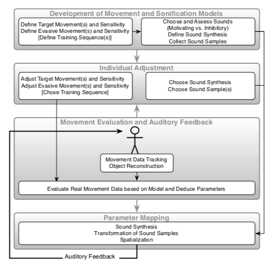
Using a tracking system, the human body is detected and its data is used to synthesize and / or transform audio files. This provides the patient with auditory feedback, which allows him to understand whether the exercise was performed correctly or not.

Here is their statement about the project:

“In PhysioSonic, we focus on the following principles: 

  • The tracking is done without a disturbance of the subject, as markers are fixed to an overall suit (and the subject does not, e.g., have to hold a device).
  • In collaboration with a sport scientist, positive (target) and negative (usually evasive) movement patterns are defined. Their range of motion is adapted individually to the subject. Also, a whole training sequence can be pre-defined.
  • The additional auditory feedback changes the perception including the proprioception of the subject, and the move- ments are performed more consciously. Eyes-free condi- tion for both the subject and an eventual observer (trainer) free the sight as an additional modality. In addition to the target movement, pre-defined evasive movements are made aware.
  • We sonify simple and intuitive attributes of the body move- ment (e.g., absolute height, velocity). Thus, the subject eas- ily understands the connection between them and the sound. This understanding is further enhanced by using simple me- taphors: e.g., a spinning-wheel-metaphor keeps the subject moving and thus ’pushing’ the sound; if the subject does not accumulate enough ’energy’, the looping sound of a disk- getting-stuck metaphor is used.
  • The sounds are adapted to each subject. Music and spoken text that are used as input sounds can be chosen and thus en- hance the listening pleasure. Also, the input sounds change over time and have a narrative structure, where the repeti- tion of a movement leads to a different sound, thus avoiding fatigue or annoyance. (Still, the sonification design is well-defined, and the quality of the sound parameters changes according to the mapping.) “

The tracking system used is the VICON tracking system that allows a spatial resolution in the millimeter range and a temporal resolution and reaction time less than 10 ms. This means that it detects movements really precisely.

The data is then processed in the VICON system and used in SuperCollider (platform for audio synthesis and algorithmic composition) to synthesize and process sounds. The system allows a very detailed continuous temporal and spatial control of the sound produced in real time.

[1]

Some videos can be found at https://iem.at/Members/vogt/physiosonic

Currently, this system is set up at the hospital Theresienhof in Frohn- leiten, Austria. 

Reference:

[1] K. Vogt, D.Pirro ́, I. Kobenz, R. Höldrich, G. Eckel – Physiosonic – Movement sonification as auditory feedback. 2009.