by Johannes Lechner - July 16, 2021July 16, 2021

ML Sample Generator Project | Phase 2 pt3

Convolutional Networks

Convolutional networks include one or more convolutional layers. These layers are typically used for feature extraction. Stacking multiple on top of each other often can extract very detailed features. Depending on the input shape of the data, convolutional layers can be one- or multidimensional, but are usually 2D as they are mainly used for working with images. The feature extraction can be achieved by applying filters to the input data. The image below shows a very simple black and white (or pink & white) image with a size 3 filter that can detect vertical left-sided edges. The resulting image can then be shrinked down without losing as much data as reducing the original’s dimensions would.

2D convolution with filter size 3 detecting vertical left edges

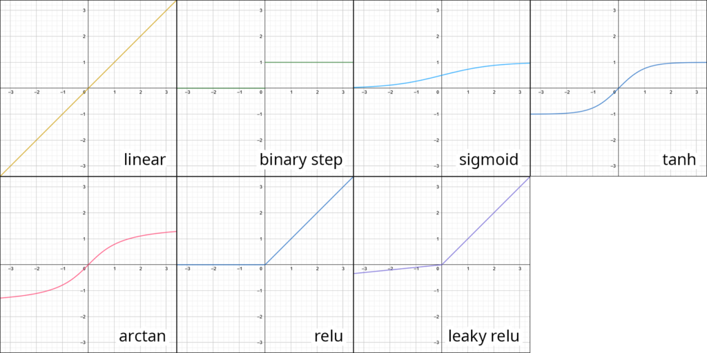
In this project, all models containing convolutional layers are based off of WavGAN. For this cutting the samples down to a length of 16384 was necessary, as WavGAN only works with windows of this size. In detail, the two models consist of five convolutional layers, each followed by a leaky rectified linear unit activation function and one final dense layer afterwards. Both models were again trained for 700 epochs.

Convolutional Autoencoder

The convolutional autoencoder produces samples only in the general shape of a snare drum. There is an impact and a tail but like the small autoencoders, it is clicky. In contrast to the normal autoencoders, the whole sound is not noisy though but rather a ringing sound. The latent vector does change the sound but playing the sound to a third party would not result in them guessing that this should be a snare drum.

Ringy conv ae sample

GAN

The generative adversarial network worked much better than the autoencoder. While still being far from a snare drum sound, it produced a continuous latent space with samples resembling the shape of a snare drum. The sound itself however very closely resembles a bitcrushed version of the original samples. It would be interesting to develop this further as the current results suggest that there is just something wrong with the layers, but the network takes very long to train which might be due to the need of a custom implementation of the train function.

Bitcrushed sounding GAN sample

Variational Autoencoder

Variational autoencoders are a sub-type of autoencoders. Their big difference to a vanilla autoencoder is the encoder’s last layer, the sampling layer. With this, variational autoencoders always provide a continuous latent space, which is much better for generative models than just to sample from what has been provided. This is achieved by having the encoder output two different vectors instead of one: one for standard deviation and one for the mean. This provides a distribution rather than a single point, leading to the decoder learning that an area is responsible for a feature and not a single sample.

Training the variational autoencoder was especially troublesome as it required a custom class with it’s own train step function. The difficulty with this type of model is that the right mix between reconstruction loss and kl loss has to be found, otherwise the model produces unhelpful results. The currently trained models all have a ramp up time of 30,000 batches until full effect of the kl loss. This value gets multiplied by a different actor depending on the model. The trained versions are with a factor of 0.01 (A), 0.001(B), as well as 0.0001(C). Model A produces a snare drum like sound, but is very metallic. Additionally instead of having a continuous latent space, the sample does not change at all. Model B produces a much better sample but still does not include much changes. The main changes are the volume of the sample as well as it getting a little bit more clicky towards the edges of the y axis. Model C has much more different sounds, but the continuity is more or less not present. In some areas the sample seems to get slightly filtered over one third of the vector’s axis but then rapidly changes the sound multiple times over the next 10%. But still, out of the three variational autoencoders model C produced the best results.

VAE with 0.01 contribution (A) sample

VAE with 0.001 contribution (B) sample

VAE with 0.0001 contribution (C) sample

Next Steps

As I briefly mentioned before, this project will ultimately run on a web server which means the next steps will be deciding how to run this app. Since all of the project has been written in python so far Django would be a good solution. But since TensorFlow offers a JavaScript Library as well this is not the only possible way to go. You will find out more about this in the next semester.

by Johannes Lechner - July 16, 2021July 16, 2021

ML Sample Generator Project | Phase 2 pt2

Autoencoder Results

As mentioned in the post before I have trained nine autoencoders to (re)produce snare drum samples. For easier comparison I have visualized the results below. Each image shows the location of all ~7500 input samples.

Rectified Linear Unit

All three graphics portray how the samples are mostly close together but some are very far out. A continuous representation is with all three models not possible. Reducing the latent vector’s maximum on both axes definitely helps, but even then the resulting samples are not too pleasing to hear. The small network has clicks in the beginning and generates very silent but noisy tails after the initial impact. The medium network includes some quite okay samples but moving around in the latent space often produces similar but less pronounced issues as the small network. And the big network produces the best sounding samples but has no continuous changes.

Clicky small relu sample

Noisy medium relu sample

Quite good big relu sample

Hyperbolic Tangent

These three networks each produce different patterns with a cluster at (0|0). The similarities between the medium and the big network lead me to believe that there is a smooth transition between random noise, to forming small clusters, to turning 45° clockwise and refining the clusters when increasing the number of trainable parameters. Just like the relu version, the reproduced audio samples of the small network contain clicks. The samples are however much better. The medium sized network is the best one out of all the trained models. It produces mostly good samples and has a continuous latent space. One issue is however that there are still some clicky areas in the latent space. The big network is the second best overall as it mostly lacks a continuous latent space as well. The produced audio samples are however very pleasing to hear and resemble the originals quite well.

Clicky small tanh sample

Close-to-original medium tanh sample

Close-to-original big tanh sample

Sigmoid

This group shows a clear tendency to cluster up the more trainable parameters exist. While in the above two groups the medium and the big network produced better results, in this case the small network is by far the best. The big network delivers primarily noisy audio samples and the medium network very noisy ones as well but they are better identifiable as snare drum sounds. The small network has by far the closest sounds to the originals but produces clicks at the beginning as well.

Clicky small sigmoid sample

Noisy medium sigmoid sample

Super noisy big sigmoid sample

In the third part of this series we will take a closer look at the other models.

by Johannes Lechner - July 16, 2021July 16, 2021

ML Sample Generator Project | Phase 2 pt1

A few months ago I already explained a little bit about machine learning. This was because I started working on a project involving machine learning. Here’s a quick refresh on what I want to do and why:

Electronic music production often requires gathering audio samples from different libraries, which, depending on the library and on the platform, can be quite costly as well as time consuming. The core idea of this project was to create a simple application with as few as possible parameters, that will generate a drum sample for the end user via unsupervised machine learning. The interface’s editable parameters enable the user to control the sound of the generated sample and a drag-and-drop space could map a dragged sample’s properties to the parameters. To simplify interaction with the program as much as possible, the dataset should only be learned once and not by the end user. Thus, the application would work with the models rather than the whole algorithm. This would be a benefit as the end result should be a web application where this project is run. Taking a closer look at the machine learning process, the idea was to train the network in the experimentation phase with snare drum samples from the library noiiz. With as many different networks as possible, this would then create a decently sized batch of models from which the best one could be selected for phase 3.

So far I have worked with four different models in different variations to gather some knowledge on what works and what does not. To evaluate them I created a custom GUI.

The GUI

Producing a GUI for testing purposes was pretty simple and straight-forward. Implementing a Loop Play option required the use of threads, which was a little bit of a challenge but working on the Interface was possible without any major problems thanks to the library PySimpleGUI. The application worked mostly bug free and enabled extensive testing of models and also already saving some great samples. However, as it can be seen below, this GUI is only usable for testing purposes and does not meet the specifications developed in the first phase of this project. For the final product a much simpler app should exist and instead of being standalone it should run on a web server.

Autoencoders

An autoencoder is an unsupervised learning method where input data is encoded into a latent vector (therefore the name autoencoder). To get from the input to the latent vector multiple dense layers reduce the dimensionality of the data, creating a bottleneck layer and forcing the encoder to get rid of less important information. This results in data loss but also in a much smaller representation of input data. The latent vector can then be decoded back to produce a similar data sample to the original. While training an autoencoder, the weights and biases of individual neurons are modified to reduce data loss as much as possible.

In this project autoencoders seemed to be a valuable tool as audio samples, even though as short as only 2 seconds, can add up to a huge size. Training with an autoencoder would reduce this information down to only a latent vector with a few dimensions and the trained model itself, which seems perfect for a web application. The past semester resulted in nine different autoencoders, each containing dense layers only. All autoencoders differ from each other by either the amounts of trainable parameters, or the activation functions, or both. The chosen activation functions are rectified linear unit, hyperbolic tangent and sigmoid. These are used in all of the layers of the encoder as well as all layers of the decoder except for the last one to get back to an audio sample (where individual data points are positive and negative).

Additionally, the autoencoders’ size (as in the amount of trainable parameters) is one of the following three:

Two dense layers with units 9 and 2 (encoder) or 9 and sample length (decoder) with trainable parameters
Three dense layers with units 96, 24 and 2 (encoder) or 24, 96 and sample length (decoder) with trainable parameters
Four dense layers with units 384, 96, 24 and 2 (encoder) or 24, 96, 384 and sample length (decoder) with trainable parameters

Combining these two attributes results in nine unique models, better understandable as a 3×3 matrix as follows:

	Small (2 layers)	Medium (3 layers)	Big (4 layers)
Rectified linear unit	Ae small relu	Ae med relu	Ae big relu
Hyperbolic tangent	Ae small tanh	Ae med tanh	Ae big tanh
Sigmoid	Ae small sig	Ae med sig	Ae big sig

All nine of the autoencoders above have been trained on the same dataset for 700 epochs. We will take a closer look on the results in the next post.

by Johannes Lechner - July 3, 2021

Harmor

The Basics

The picture above shows Harmor’s interface. We can group the Interface into three sections: The red part, the gray part and the window to the right. Firstly, the easiest section to understand is the window to the right. Harmor is an additive synthesizer, which means the sounds it generates are made up of sine waves added on top of each other. The window on the right displays the frequencies of the individual sine waves, played over the last few seconds. Secondly, the red window is where most of the sound is generated. There are different sections and color-coded knobs to be able to identify what works together. Left of the center you can see an A/B switch. The red section exists twice: once for state A and once for state B. These states can be mixed together via the fader below. Lastly the gray area is for global controls. The only exception is the IMG tab, which we will cover a little later. As you can see there are many knob, tabs and dropdowns. But in addition to that most most of the processing can be altered with envelopes. These allow the user to draw a graph with infinitely many points to either use it as an ADSR curve, an LFO, or map it to keyboard, velocity, X, Y & Z quick modulation and more. At this point it already might become clear that Harmor is a hugely versatile synth. It’s marketed as an additive / subtractive synthesizer and features an immense amount of features which we will take a closer look at now.

Additive or Subtractive?

As mentioned above Harmor is marketed as an additive / subtractive synthesizer. But what does that mean? While Harmor is built using additive synthesis as its foundation, the available features closely resemble a typical subtractive synth. But because Harmor is additive, there are no audio streams being processed. Instead a table of frequency and amplitude data is manipulated resulting in an efficient, accurate and partly very unfamiliar and creative way to generate audio streams. Harmor features four of these additive / subtractive oscillators. Two can be seen on the image above in the top left corner. These can be mixed in different modes and then again mixed with the other two via the A/B switch. In addition to the four oscillators, Harmor is also able to synthesize sound from the IMG section. The user can drag-and-drop audio or image files in and Harmor can act like a sampler, re-synthesizing audio or even generating audio from images drawn in Photoshop.

The Generator Section

As you can see in addition to the different subsections being walled in by dotted lines, this section is color coded as well. The Timbre section allows you to select any waveform by again drawing and then morphing between two of them with different mixing modes. Harmor allows you to import a single cycle waveform to generate the envelope. But you can import any sample and generate a waveform from it. Here is an example where I dragged a full song into it and processed it with the internal compressor module only:

The blur module allows you to generate reverb-like effects and also preverb. Tremolo generates the effect of a stereo vibrato, think about jazz organs. Harmonizer clones existing harmonics by the offset/octaves defined. And prism shifts partials away from their original relationship with the fundamental frequency. A little prism usually generates a detune-like effect, more usually metallic sounds. And here is the interesting part: As with many other parameters as well, you can edit the harmonic prism mapping via the envelopes section. This allows you to create an offset to the amount knob on a per frequency basis. Here is an example of a usage of prism:

As you can see in the analyzer on the right: There is movement over time. In the Harmonic prism envelope I painted a graph so that the knob does not modify lower frequencies but only starts at +3 octaves.
The other options from this section, unison, pitch, vibrato and legato should be clear from other synthesizers.

The Filter Section

As seen above, Harmor features two filters per state. Each filter can have a curve selected from the presets menu. The presets include low pass, band pass, high pass and comb filtering. Additionally you can draw your own curve as explained in the Basics section above. The filters can additionally be control the mix for the envelope, keyboard tracking, width, actual frequency and resonance. But the cool thing is how these filters are combined: The knob in the middle lets you fade between only filter 2, parallel processing, only filter 1, filter 1 + serial processing and serial processing only. In the bottom half there is a one-knob pluck knob as well as a phaser module with, again, custom shaped filters.

The Bottom Section

As you can see above the bottom section features some general global functions. On the left side most should be clear. The XYZ coordinate grid offers a fast way to automate many parameters by mapping them to either X Y or Z and then just editing events in the DAW. On the top right however there are four tabs that open new views. Above we have seen the ENV section where you can modulate about anything. The green tab is the image tab. We already know that Harmor can generate sound from images and sound (not that this is a different way of using existing sound, before I loaded it into an oscillator, now we are talking about the IMG tab). On the right you can see a whole lot of knobs, some of them can be modified by clicking in the image. C and F are course and fine playback speed adjustments, time is the time offset. The other controls are used to change how the image is interpreted and partially could be outsourced to image editors. I’m going to skip this part, as this post would get a whole lot more complicated if not. It would probably be best to just try it out yourself.

The third tab contains some standard effects. These are quite good but especially the compressor stands out as it rivals the easy-but-usefullness of OTT.

And finally, the last section: Advanced (did you really think this was advanced until now? :P) Literally the whole plugin can be restructured here. I usually only go in here to enable perfect precision mode, threaded mode (enables multi core processing) and high precision image resynthesis. Most of these features are usually not needed and seem more like debugging features so I will not go into detail about them, but like before I encourage you to try it out. Harmor can be very overwhelming and as many people mention in reviews: “Harmor’s biggest strength is also it’s greatest weakness, and probably why there are so few reviews for such an amazing synth. You can use Harmor for years, and still feel like a noob only scratching the surface. That makes writing a review difficult. How can you give an in-depth review, when you feel so green behind the ears? You only need to watch a few YT videos (e.g. Seamless) or chat with another user to discover yet another side to this truly versatile beast.”

Harmor on KVR ⬈
Harmor on Image-Line ⬈
Harmor Documentation ⬈ (a whole lot more details and a clickable image if you have more detailed questions)

by Johannes Lechner - March 14, 2021March 21, 2021

Processing Audio Data for Use in Machine Learning with Python

I am currently working on a project where I am using machine learning to generate audio samples. One of the steps involved is pre-processing.

What is pre-processing?

Pre-processing is a process where input data somehow gets modified to be more handleable. An easy everyday life example would be packing items in boxes to allow for easier storing. In my case, I use pre-processing to make sure all audio samples are equal before further working with them. By equal, in this case I mean same sample rate, same file type, same length and same time of peak. This is important because having a huge mess of samples makes it much harder for the algorithm to learn the dataset and not just return random noise but actually similar samples.

The Code: Step by step

First, we need some samples to work with. Once downloaded and stored somewhere we need to specify a path. I import os to store the path like so:

import os

PATH = r"C:/Samples"

DIR = os.listdir( PATH )

Since we are already declaring constants, we can add the following:

ATTACK_SEC = 0.1

LENGTH_SEC = 0.4

SAMPLERATE = 44100

These are the “settings” for our pre-processing script. The values depend strongly on our data so when programming this on your own, try to figure out yourself what makes sense and what does not.

Instead of ATTACK_SEC we could use ATTACK_SAMPLES as well, but I prefer to calculate the length in samples from the data above:

import numpy as np

attack_samples = int(np.round(ATTACK_SEC * SAMPLERATE, 0))

length_samples = int(np.round(LENGTH_SEC * SAMPLERATE, 0))

One last thing: Since we usually do not want to do the pre-processing only once, form now on everything will run in a for-loop:

for file in DIR:

Because we used the os import to store the path, every file in the directory can now simply accessed by the file variable.

Now the actual pre-processing begins. First, we make sure that we get a 2D array whether it is a stereo file or a mono file. Then we can resample the audio file with librosa.

import librosa

import soundfile as sf

try:

data, samplerate = sf.read(PATH + "/" + file, always_2d = True)

except:

continue

data = data[:, 0]

sample = librosa.resample(data, orig_sr=samplerate, target_sr=SAMPLERATE)

The next step is to detect a peak and to align it to a fixed time. The time-to-peak is set by our constant ATTACK_SEC and the actual peak time can be found with numpy’s argmax. Now we only need to compare the two values and do different things depending on which is bigger:

peak_timestamp = np.argmax(np.abs(sample))

if (peak_timestamp > attack_samples):

new_start = peak_timestamp – attack_samples

processed_sample = sample[new_start:]

elif (peak_timestamp < attack_samples):

gap_to_start = attack_samples – peak_timestamp

processed_sample = np.pad(sample, pad_width=[gap_to_start, 0])

else:

processed_sample = sample

And now we do something very similar but this time with the LENGTH_SEC constant:

if (processed_sample.shape[0] > length_samples):

processed_sample = processed_sample[:length_samples]

elif (processed_sample.shape[0] < length_samples):

cut_length = length_samples – processed_sample.shape[0]

processed_sample = np.pad(processed_sample, pad_width=[0, cut_length])

else:

processed_sample = processed_sample

Note that we use the : operator to cut away parts of the samples and np.pad() to add silence to either the beginning or the end (which is defined by the location of the 0 in pad_width=[]).

With this the pre-processing is done. This script can be hooked into another program right away, which means you are done. But there is something more we can do. The following addition lets us preview the samples and the processed samples both via a plot and by just playing them:

import sounddevice as sd

import time

import matplotlib.pyplot as plt

#PLOT & PLAY

plt.plot(sample)

plt.show()

time.sleep(0.2)

sd.play(sample)

sd.wait()

plt.plot(processed_sample)

plt.show()

time.sleep(0.2)

sd.play(processed_sample)

sd.wait()

Alternatively, we can also just save the files somewhere using soundfile:

sf.write(os.path.join(os.path.join(PATH, "preprocessed"), file), processed_sample, SAMPLERATE, subtype='FLOAT')

And now we are really done. If you have any comments or suggestions leave them down below!

by Johannes Lechner - January 10, 2021January 19, 2021

Audio & Machine Learning (pt 3)

Part 3: Audio Generation using Machine Learning

Image processing and generating using machine learning has been significantly enhanced by using deep neural networks. And even pictures of human faces can now be artificially created as shown on thispersondoesnotexist.com. Images however are not that difficult to analyse. A 1024px-by-1024px image, as shown on thispersondoesnotexist, has “only” 1,048,576 pixels; split into three channels that is 3,145,728 pixels. Now, comparing this to a two-second-long audio file. Keep in mind that two seconds really can not contain much audio – certainly not a whole song but even drum samples can be cut down with only two seconds of playtime. An audio file has usually a sample rate of 44.1 kHz. This means that one second audio contains 44,100 slices, two seconds therefor 88,200. CD quality audio wav files have a bit depth of 16bit (which today is the bare minimum in digital audio workstations). So, a two second audio file has 2¹⁶ * 88,200 samples which results in 22,579,200 samples. That is a lot. But even though music or in general audio generation is a very human process and audio data can get very big very fast, machine learning can already provide convincing results.

Midi

Before talking about analysing audio files, we have to talk about the number one workaround: midi. Midi files only store note data such as pitch, velocity, and duration, but not actual audio. The difference in file size is not even comparable which makes midi a very useful file type to be used in machine learning.

FlowMachines is one of the more popular projects that work with midi. It is a plugin for DAWs that can help musicians generate scores. Users can choose from different styles to sound like for example the Beatles. These styles correspond to different trained models. FlowMachine works so well that there is already commercial music produced by it. Here is an example of what it can do:

Audio

Midi generation is a very useful helper, but it will not replace musicians. Generating audio on the other hand could potentially do that. Right now, generating short samples is the only viable way to go and it is just in its early stages but still, that could replace sample subscription services one day. One very recently developed architecture that seems to deliver very promising results is the GAN.

Generative Adversarial Networks

A generative adversarial network (GAN) simultaneously trains two models rather than one: A generator which trains with random values and captures the data distribution, and a discriminator which estimates the probability that a sample came from the training data rather than the generator. Through backpropagation both networks continuously enhance each other which leads to the generator getting better at generating fake data and the discriminator getting better at finding out whether the data came from the training data or the generator.

An already very sophisticated generative adversarial network for audio generation is WaveGAN. It can train on audio examples with up to 4 seconds in length at 16kHz. The demo includes a simple drum machine with very clearly synthesized sounds but shows how GANs might be the right direction to go. But what GANs really have to offer is the parallel processing shown in GANSynth. Instead of predicting a single sample at a time which autoregressive models are pretty good at, GANSynth can process multiple sequences in parallel making it about 50,000 times faster than WaveNet.

https://magenta.tensorflow.org/gansynth
https://github.com/chrisdonahue/wavegan
https://www.musictech.net/news/sony-flowmachines-plug-in-uses-ai/

by Johannes Lechner - December 20, 2020January 19, 2021

Audio & Machine Learning (pt 2)

Part 2: Deep Learning

Neural Networks

Neural networks are a type of machine learning which are inspired by the human brain and consist of many interconnected nodes (neurons). The goal of using neural networks is to train a model, which is a file that is or has been trained by machine learning algorithms to recognize certain properties or patterns. Models are trained with a set of data and once trained they can be used to make predictions about new data. A neural network is split into different layers, to which diffident Neurons belong to. The layers a neural network consists of are an input layer, an output layer and one or more hidden layers in between. Mathematically, a neuron’s output can be described as the following function:

ƒ( w^T x + b)

In the function above w is a weight vector, x is a vector of inputs, b is a bias and ƒ is a nonlinear activation function. When a neural network is training, weights w and biases b modify the model to better describe a set of input data (a dataset). Multiple inputs then result in a sum of weighted inputs.

∑_i w_i x_i + b = w₁ x₁ + w₂ x₂ + … + w_n x_n + b

The neurons take a set of such weighted inputs and through an activation function produce new values.

Training

When training the network analyzes the individual packs of data (examples) from the dataset and initializes the weights of its neurons with random values and the bias with zero. Neural network training consists of three parts: A loss function evaluates how well the algorithm models the dataset. The better the predictions are the smaller the output of the loss function becomes. Backpropagation is the process of applying gradients to weights. The output of the loss function is used to calculate the difference between the current value and the desired value. The error is then sent back layer by layer from the output to the input and the neurons’ weights get changed depending on their influence on the error. Gradients are used to adjust the neurons’ weights based on the output of the loss function. This is done by checking how the parameters have to change to minimize loss (= decrease the output of the loss function). To modify the neurons’ weights, the gradients multiplied by a defined factor (the learning rate) are subtracted from the weights. This factor is very small (like 0.001) to ensure weight changes remain small to not jump over the ideal value (close to zero).

Layers

As mentioned above, a neural network consists of multiple layers, which are groups of neurons. One or more are hidden layers. These calculate new values for previous values with a specific function (activation function).

Hidden layers can be of various types like linear or dense layers and the type of the layer determines what calculations are made. As the complexity of the problems increases the complexity of the functions must also increase. But stacking multiple linear layers in sequence of each other would be redundant as this could be written out as one function. Dense layers exist for this reason. They can approximate more complex functions which make use of activation functions. Instead of only for the input values, activation functions are applied on each layer which in addition to more complexity leads also to more stable and faster results.

The following list introduces some commonly used activation functions:

linear (input=output)
binary step (values are either 0 or 1)
sigmoid (s-shaped curve with values between 0 and 1 but never 0 and 1)
tanh (like the sigmoid but maps from -1 to 1)
arcTan (maps the input to values between -pi/2 to +pi/2)
reLU – Rectified Linear Unit (sets any negative values to 0)
leaky reLU (does not completely remove negative values but drastically lowers their magnitude)

activation functions displayed in Geogebra

Deep Learning

As mentioned before, there are different layers in a neural network. What was not mentioned is that a neural network with more than one hidden layer is called a deep neural network. Thus the process of training a deep neural network’s model is called deep learning. Deep neural networks have a few advantages to neural networks. As mentioned above activation functions introduce non-linearity. And having many dense layers stacked after each other leads to being able to compute much more complex problem’s solutions. Including audio (finally)!

http://www.deeplearningbook.org
https://www.techradar.com/news/what-is-a-neural-network
https://www.ibm.com/cloud/learn/neural-networks
https://www.mygreatlearning.com/blog/activation-functions/
https://algorithmia.com/blog/introduction-to-optimizers
https://medium.com/datathings/neural-networks-and-backpropagation-explained-in-a-simple-way-f540a3611f5e
https://medium.com/datathings/dense-layers-explained-in-a-simple-way-62fe1db0ed75
https://medium.com/deeper-learning/glossary-of-deep-learning-batch-normalisation-8266dcd2fa82
https://semanti.ca/blog/?glossary-of-machine-learning-terms

by Johannes Lechner - December 13, 2020January 19, 2021

Audio & Machine Learning (pt 1)

Part 1: What is Machine Learning?

Machine Learning is essentially just a type of algorithm that improves over time. But instead of humans adjusting the algorithm the computer does it itself. In this process, computers discover how to do something without being programmed to do so. The benefits of such an approach to problem solving is that algorithms too complex for humans to develop can be learned by the machine. This leads to programmers being able to focus on what goes in to and what out of the algorithm rather than the algorithm itself.

Approaches

There are three broad categories of machine learning approaches:

Supervised Learning
Unsupervised Learning
Reinforcement Learning

Supervised learning is used for figuring out how to get from an input to an output. Inputs are classified meaning the dataset (or rather trainset, the part of the dataset used for training) is already split up into categories. The goal of using supervised learning is to generate a model that can map inputs to outputs. An example would be automatic audio file tagging – like either drum or guitar.

Unsupervised learning is used when the input data has not been labelled. The algorithm has to find out on its own how to describe a dataset. Common use cases are feature learning and discovering patterns in data (which might not have been visible without machine learning).

Reinforcement learning is probably what you have seen on YouTube. These are the algorithms that interact with something (like a human would do with a controller for example) and is either punished or rewarded for its behavior. Algorithms learning to play Super Mario World or Tesla’s Autopilot are trained with reinforcement learning.

Of course, there are other approaches as well, but these are a minority, and it is easier to just stick with the three categories above.

Models

The process of machine learning is to create an algorithm which can describe a set of data. This algorithm is called a model. A model exists from the beginning on and is trained. Trained models can then be used for example to categorize files. There are various approaches to machine learning:

Classifying
Regression
Clustering
Dimensionality reduction
Neural networks / deep learning

Classifying models are used to (you guessed it) classify data. They predict the type of data which can be several options (for example colors). One of the simplest classifying models is a decision tree which follows a flowchart-like concept of asking a question and getting either yes or no as an answer (or in more of a programmer’s terms: if and else statements). If you think of it as a tree (the way it is meant to be understood) you start at the root with one question, then get on to a branch where the next question is until you reach a leaf, which represents the class or tag you want to assign.

Regression models come from statistical analysis. There are a multitude of regression models, the easiest of which is the linear regression. Linear regression tires to describe a dataset with just one liner function. The data is mapped on to a 2-dimensional space and then a linear function which “kind of” fits all the data is drawn. An example for regression analysis would be Microsoft Excel’s trendline tool.

non-linear regression | from not enough learning (left) to overfitting (right)

Clustering is used to group similar objects together. If you have unclassified data and want to make use of supervised learning, regression models can automatically classify the objects for you.

Dimensionality reduction models (again an aptronym) reduce dimensionality of the dataset. The dimensionality is the number of variables used to describe a dataset. As usually different variables do not contribute equally to the dataset, the dataset can still be reliably described by less variables. One example for dimensionality reduction is the principal component analysis. In 2D space the PCA generates a best fitting line, which is usually where the least squared distance from the points to the line is.

2D principal component analysis | the ideal state would be when the red lines are the smallest

Deep Learning will be covered in part 2 of this series as this is the main focus of this series.

https://en.wikipedia.org/wiki/Glossary_of_artificial_intelligence
https://www.educba.com/machine-learning-models/
https://www.educba.com/machine-learning-algorithms/

by Johannes Lechner - December 6, 2020December 6, 2020

Mechanical & Performance Royalties: What the hell is that?

As an independent artist you probably have your music on Spotify & co. And these services pay you through your aggregator, distributor or label. Additionally you might DJ or do some public performances where you get paid. But did you know that you are owed more than that? Platforms like Spotify and venues where you play are required by law to pay a fee to so-called collection societies. And these collection societies get the money whether you’ve joined or not.

Artist vs. Writer

Before talking about the different types of revenue that can be collected we first need to know that there are two types of musicians: songwriters and performing artists. The artist or performer is the entity performing the song. Take Martin Garrix for example: When releasing a track you always hear about “Martin Garrix”. But that’s not his real name, that’s his artist name or performer name. But as a songwriter he has to state his real name which would be Martijn Gerard Garritsen. On tracks like “Animals” only Martin himself worked on it so the difference is really not important, but bands or other artists have many different people working on one song. While the artists on “Titanium” are David Guetta and Sia, the songwriters are many more people who usually you do not know. And these people get money as well.

Performance Royalties

Performing artists hold the copyrights to the recording of a song. This is called a master recording. The royalties are paid to the artists every time a song is performed in public. This means a public performance is whenever your song is played in a bar, over the radio or on streaming services.

Mechanical Royalties

Songwriters (incl. Texters) hold the copyright to the melody and lyrics of a song. The royalties are paid whenever someone acquires a copy of a song. This can be online (e.g. through iTunes) or on physical media (e.g. CDs).

How to get paid

The two rights described above will both be collected via collection societies. You can either work with them directly or use a label or publisher. But in both cases you need to sign up with the societies, which usually costs money!

Direct approach

In Austria the performance royalties are collected by AKM, the mechanical ones by AUME. These two work together so you only have to sign up once and you can use only one platform to tell them about your work. Singing up costs a fee but fortunately in Austria that’s a one time thing. If you live somewhere else there might be a one time fee, an ongoing fee or both (like in Germany). Then you will add all your tracks to their database. Mechanical royalties will be automatically collected, but whenever you play something live you will either be asked by someone from the venue to give them a tracklist, or you will send the tracklist directly to your PRO (=Performance Rights Organization).

3rd-party approach

If you want you can sign up with 3rd parties to get some bonus features. This mostly applies to song copyrights where you can have your own publisher. Master recordings are usually handled be the record label (which you might be yourself).

Music publishers take a percentage cut off of your income from royalties but make submitting your music a little easier and more importantly pitch your songs! Depending on your publisher and your contract this can mean just adding it to a database and having to manually apply for synch (synch means your music being played in a TV ad for example). Or it can mean that you really don’t have much work to do and money is arriving on it’s own.

Stuff to check out

If you are new to all of this you might want to check out this Q&A by AKM: https://www.akm.at/mitglieder/fragen-antworten (German)

Here you can sign up for AKM & AUME (highly recommended!): https://www.akm-aume.at/akm-webapp/ (German again)

Other than performance and mechanical royalty laws, there is also neighbouring rights. Basically you will get money if you are an artist, a label and a music video creator. Here’s the Austrian site: http://lsg.at/ (danger! bad design!) and this one is for artists specifically https://www.lsg-interpreten.com/ (both in German). If you want to learn more about neighbouring rights I’d recommend checking out the German society GVL though: https://www.gvl.de/ (German & English)

If you have questions or anything to add I’d love to hear from you in the comments. Happy royalty collecting!

by Johannes Lechner - November 29, 2020December 6, 2020

How to get your music onto FM4

Or in other words: How to correctly pitch your songs to professionals

Due to a recent achievement, which is having my newest song being played on radio FM4 multiple times and giving an interview on it, i thought I’d share my knowledge.

Tools that help pitching

Before talking about pitching to FM4 or in general to radio stations, I’d like to show you two of the most known alternative options, which require far less work.

SubmitHub

This site lets you submit to bloggers, labels, YouTubers, playlisters, influencers and radio stations (small ones though). When creating your account you get a few credits which then can be spent on different people and networks – usually the bigger ones cost a little more. This site might look overwhelming at first but has a lot of great features! Unfortunately, you can’t really send your music to many outlets without purchasing some premium credits. The average approval rate on standard credits is 4%, as opposed to 18% on premium. So, the free credits don’t do as well but still, they do something. And if you only want to target a specific YouTube channel for example this would be perfectly sufficient.

LabelRadar

In contrary to SubmitHub, LabelRadar is far more minimalistic and easy-to-use. Now, don’t get fooled by the name – of course you can send your music to labels, but to promoters as well! Like the previous one, this website gives you a few credits when you start out, but you can send you music into a general pool where the labels or promoters don’t get notified but can browse through. And if you spend all of your credits, they will send you 5 new ones once a month.

Pitching to big radio stations

Okay, so get your pen and paper ready – you’ll want to follow this as closely as possible. I have heard of cases where radio stations did not listen to a track simply because it was in a zip file. This is understandable considering they have to listen to huge amounts of tracks every day. So, as artists it is our job to make it as easy as possible for them to listen to our songs. And we can do that with email and a link to a Dropbox folder. More on that later. Below is a list of what you need but I will get into detail anyway.

the song (obviously)
artwork
either a classic Press Kit
or an EPK
professional press photos

The song

Obviously your song has to fit in the radio station’s program. Ideally you have heard something similar in the past few weeks, which is something you can then refer to in your email. In your Dropbox folder add the file as an mp3 and as a wav (one for listening and one for actually airing it). Be sure to add as many id3 tags as possible. This can be done with software like AudioShell. As wav files don’t really support much tagging I always provide a flac file as well so that the tags appear as well as it being a lossless file. If your mp3 is smaller than 10MB (with id3 tags) then you can add it as an attachment to your email.

Artwork

The most important Artwork is your cover – including this is a must. Any other stuff you have might work as well. Don’t add your “coming soon” banners, but if you have a Spotify Canvas or something then they might look at it and maybe even share it.

Classic press kit

This is a one page A4 document containing all the information for your release. At the beginning of the press kit you’ll want to show all the basic info like your release title, cover, artist name, release date, label name, IRSC and UPC/EAN. Then add a short biography and a list of previous releases. Finally add some contact info. In my case including my phone number resulted in a spontaneous call where we did an interview.

Here is an example showing the press kit for my latest release “With You”:

Press Kit for “With You” – right click -> view image to make it bigger

And one more thing: don’t shift the design around too much. The radio stations will want to open a press kit and just look at a certain point rather than searching for the info!

EPK

EPK stands for electronic press kit. If you have a classic press kit you won’t need an EPK but I usually to do both. Essentially the EPK is the same as a classic press kit, but it being online comes with a few advantages: You can embed your music and let it autoplay when opening the webpage. Your songs can directly be downloaded with a button. And you can make fancy galleries with your press photos!

Here is an example, again for “With You”:

Screenshot of my EPK for “With You”right click -> view image to make it bigger

Whether you want to offer the complete song as a download or not is up to you. If you are concerned about other people finding this page and downloading your music I have a suggestion for you: Either you use a file sharing service and just don’t offer it on your site. Or you do the more elegant way and use some PHP coding / WordPress plugin installing. I’m using Members to create a custom group for press, promoters, etc. Then I’ll set up a temporary login link for that user group. Finally, to hide the page from normal users, I’m using Visibility Logic for Elementor (and Elementor Page Builder obviously).

Press photos

There’s not much to talk about this one but be sure to have them somewhere ready to be viewed and downloaded!

The email

Now that you have all the parts prepared let’s talk about the email. The most important thing to remember is the KISS Principle (Keep It Short and Simple)! Describe your song in about one to two sentences and then add the link(s). Then thank them for listening and that’s it! As mentioned above, if your mp3 (including id3 tags like the artwork) is smaller than 10MB you can add it as an attachment.

Now about the links: If you have an EPK you should add the link to it here. The other link will be to your folder on Dropbox or other providers and this should contain the audio files, the cover, the press kit and if applicable a txt with the lyrics. I also like to include a shortcut to my EPK but this is probably not very useful as the link is already in the email.

And that’s it. If you have done everything correctly send you music about 1.5 to 2.5 weeks before the release date. And then you’ll have to play the waiting game – with a bit of luck you’ll have your music on FM4 (or any other radio station). Let me know in the comments if this was helpful to you and whether you plan to send something to a radio station or if you already had something played on air!